Download
1 / 48
480 likes | 488 Views
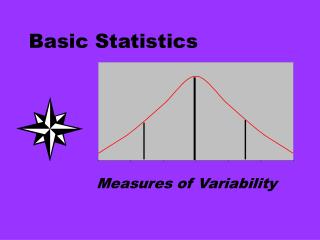
Basic statistics. Index. Measures of Central Tendency Measures of variability of distribution Covariance and Correlation Probability distribution Shape of Data Testing for normality Basics of Linear Regression Variation in Linear Regression Linear Regression Analysis Matrix Operations.

E N D
Index • Measures of Central Tendency • Measures of variability of distribution • Covariance and Correlation • Probability distribution • Shape of Data • Testing for normality • Basics of Linear Regression • Variation in Linear Regression • Linear Regression Analysis • Matrix Operations
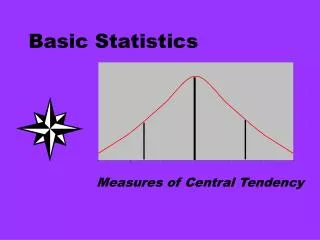
I-Measures of Central Tendency • Mean … the average score • Median … the value that lies in the middle after ranking all the scores • Mode … the most frequently occurring score
II-Variation or Spread of Distributions Measures that indicate the spread of scores: • Range • Standard Deviation
II-Variation or Spread of Distributions Range: • It compares the minimum score with the maximum score • Max score – Min score = Range • It is a crude indication of the spread of the scores because it does not tell us much about the shape of the distribution and how much the scores vary from the mean
II-Variation or Spread of Distributions • Variance – A measure of variation for interval-ratio variables; it is the average of the squared deviations from the mean
II-Variation or Spread of Distributions Why n-1? • In order to calculate an unbiased estimate of the population standard deviation, subtract one from the denominator. • Sample standard deviation tends to be an underestimation of the population standard deviation.
II-Variation or Spread of Distributions • Standard Deviation – A measure of variation for interval-ratio variables; it is equal to the square root of the variance.
Covariance and correlation measure linear association between two variables, say X and Y. Covariance: III-Covariance and Correlation: Covarianceis used to estimate the linear association between X and Y for the population.
III-Covariance and Correlation: • Let’s first note that, of all the variables a variable may covary with, it will covary with itself most strongly • In fact, the “covariance of a variable with itself” is an alternative way to define variance:
III-Covariance and Correlation: Limitation of covariance • One limitation of the covariance is that the size of the covariance depends on the variability of the variables. • As a consequence, it can be difficult to evaluate the magnitude of the covariation between two variables. • If the amount of variability is small, then the highest possible value of the covariance will also be small. If there is a large amount of variability, the maximum covariance can be large.
III-Covariance and Correlation: Correlation: • When expressed this way, the covariance is called a correlation • The correlation is defined as a standardized covariance.
Correlation measures the degree of linear association between two variables, say X and Y. There are no units – dividing covariance by the standard deviations eliminates units. Correlation is a pure number. The range is from -1 to +1. If the correlation coefficient is -1, it means perfect negative linear association; +1 means perfect positive linear association. III-Covariance and Correlation: Correlation is used with sample data to estimate the linear association between X and Y for the population.
III-Covariance and Correlation: • The value of r can range between -1 and + 1. • If r = 0, then there is no correlation between the two variables. • If r = 1 (or -1), then there is a perfect positive (or negative) relationship between the two variables.
III-Covariance and Correlation: • Advantages and uses of the correlation coefficient • Provides an easy way to quantify the association between two variables • Foundation for many statistical applications
IV-Probability Distributions • A statistical distribution is a mathematically-derived probability function that can be used to predict the characteristics of certain applicable real populations • Statistical methods based on probability distributions are parametric, since certain assumptions are made about the data
IV-Probability Distributions Binomial distribution: The binomial distribution applies to events that have two possible outcomes. The probability of r successes in n attempts, when the probability of success in any individual attempt is p, is given by:
IV-Probability Distributions Normal distrbution: • The most used continuous probability distribution: • Many observations tend to approximately follow this distribution • Bell shaped • Mean, median and mode are the same • Mean and standard deviation specify the curve
IV-Probability Distributions f(X) Changingμshifts the distribution left or right. Changing σ increases or decreases the spread. σ μ X
IV-Probability Distributions • The normal curve is not a single curve but a family of curves, each of which is determined by its mean and standard deviation. • In order to work with a variety of normal curves, we cannot have a table for every possible combination of means and standard deviations.
IV-Probability Distributions Standard normal curve: • The Standard Normal Curve (z distribution) is the distribution of normally distributed standard scores with mean equal to zero and a standard deviation of one. • A z score is nothing more than a figure, which represents how many standard deviation units a raw score is away from the mean. • Z-score is useful in comparing variables with very different observed units of measure. • Z-score allows for precise predictions to be made of how many of a population’s scores fall within a score range in a normal distribution.
IV-Probability Distributions Z score: • What we need is a standardized normal curve which can be used for any normally distributed variable. Such a curve is called the Standard Normal Curve.
IV-Probability Distributions Interpreting the graph (empirical rule)
V-Shape of Data • There are further statistics that describe the shape of the distribution, using formulae that are similar to those of the mean and variance: • 1st moment - Mean (describes central value) • 2nd moment - Variance (describes dispersion) • 3rd moment - Skewness (describes asymmetry) • 4th moment - Kurtosis (describes peaked ness)
V- shape of data Measures of asymmetry of data If skewness equals zero, the histogram is symmetric about the mean
V- Shape of data Skewness: Positive or right skewed: • There are more observations below the mean than above it • When the mean is greater than the median • Longer right tail Negative or left skewed: • There are a small number of low observations and a large number of high ones • When the median is greater than the mean • Longer left tail
Normal (skew = 0) Positive Skew Negative Skew V- Shape of data Skewness:
V- Shape of data Kurtosis Kurtosis relates to the relative flatness or peaked ness of a distribution. A standard normal distribution (blue line: µ = 0; = 1) has kurtosis = 0. A distribution like that illustrated with the red curve has kurtosis > 0 with a lower peak relative to its tails.
V- Shape of data Kurtosis • Platykurtic– When the kurtosis < 0, the frequencies throughout the curve are closer to be equal (i.e., the curve is more flat and wide) • Thus, negative kurtosis indicates a relatively flat distribution • Leptokurtic– When the kurtosis > 0, there are high frequencies in only a small part of the curve (i.e, the curve is more peaked) • Thus, positive kurtosis indicates a relatively peaked distribution
Mesokurtic (s4 = 3) Platykurtic (s4 < 3) Leptokurtic (s4 > 3) V- Shape of data Kurtosis
VI-Testing for Normality Jarque-Bera test: First we define the skewness (S) and kurtosis (K) of a set of returns: When returns are normally distributed: S=0 and K=0. The Jarque-Bera test allows us to test for normality of historical returns: This allows us to calculate the p-value: we can reject the hypothesis that returns are normally distributed with 100% (1-p) confidence Source: World Bank
VII-Linear regression • A statistical technique that uses a single, independent variable (X) to estimate a single dependent variable (Y). • Based on the equation for a line: • Y = b + mX
VII-Linear regression e = b b + Y X i 0 1 Y ? (the actual value of Yi) Yi X Xi
VII-Linear regression Population Regression Coefficients for a . . . ˆ Sample Y = b0 + b1Xi + e ˆ Y = b0 + b1Xi
VII-Linear regression ANOVA - Variation SST is a measure of the total variation of observations. A measure of the differences in observations. Due to regression SSTR SST Random/unexplained. SSE SST = SSTR + SSE
VII-Linear regression Linear Regression - Variation Y SSE =(Yi - Yi )2 _ SST = (Yi - Y)2 _ SSR = (Yi - Y)2 _ Y X Xi
_ SSy =(Yi - Y)2 _ _ SSxy =(Xi - X)(Xi - Y) SSE = S YX n-2 VII-Linear regression Determining the Regression Line/Model Manual Calculations _ _ SSE =(Yi - Yi )2 SSR = (Yi - Y)2 SST = (Yi - Y)2 _ SSx =(Xi - X)2 b1=SSxy/SSx _ _ b0 = Y – b1X MSE = SSE / df MSR = SSR / df R2 = SSR/SST t-test = b1 / Sb1
VII-Linear regression Determining the Regression Line/Model using Excel