Download
1 / 51
520 likes | 796 Views
Basic Statistics. KNES 510 Research Methods in Kinesiology. How Software is Used in Statistics. Types of software for statistics Minitab Statistical Analysis system (SAS) Statistical Package for the Social Sciences (SPSS) Predictive Analytics Software ( PASW ) Why not Microsoft Excel?

E N D
Basic Statistics KNES 510 Research Methods in Kinesiology
How Software is Usedin Statistics • Types of software for statistics • Minitab • Statistical Analysis system (SAS) • Statistical Package for the Social Sciences (SPSS) • Predictive Analytics Software (PASW) • Why not Microsoft Excel? • http://www.youtube.com/
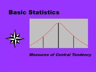
Why We Need Statistics • Statistics is an objective way of interpreting a collection of observations • Types of statistics • Descriptive • Central tendency • Variability • Correlational • Inferential • Differences within or between groups
Ways to Select a Sample • Random sampling: tables of random numbers • Stratified random sampling • Strata=small groups. Sample from each strata • Systematic sampling • Pick a start and sample every nth number. • Random assignment • Justifying post hoc explanations • Convenience sample? • How good does the sample have to be? • Good enough for our purposes!
Descriptive Statistics • Descriptive statistics are used to summarize or condense a group of scores • They include measures ofcentral tendencyand measures of variability Humans Mean=100 SD=15
Central Tendency • Measures of central tendency describe the average or common score of a group of scores • Common measures of central tendency include the mean, median,andmode
Mean • The mean is the arithmetic average of the scores • The calculation of the mean considers both the number of scores and their value • The formula for the mean of the variable X is:
Mean • Six men with high serum cholesterol participated in a study to examine the effects of diet on cholesterol • At the beginning of the study, their serum cholesterol levels (mg/dL) were: 366, 327, 274, 292, 274, 230 • Determine the mean
Calculating the Mean Using SPSS • Analyze -> Descriptive Statistics -> Frequencies command may be used to determine the mean (you will need to select the “Statistics…” button to choose the “Mean”
Median • The median is the middle point in an ordered distribution at which an equal number of scores lie on each side of it • It is also known as the 50th percentile (P50), or 2nd quartile (Q2)
Median • The position of the median (Mdn) can be calculated as follows:
Median • Example: Calculate the median for the following measurements for height: 71”, 73”, 74”, 75”, 72”
Median • Step One: Place the scores in order from lowest to highest. 71”, 72”, 73”, 74”, 75” • Step Two: Calculate the position of the median using the following formula:
Median • Step Three: Determine the value of the median by counting from either the highest or the lowest score until the desired score is reached (in this case the 3rd score)
Median • Suppose that in our previous distribution we had a sixth score as follows: 71”, 72”, 73”, 74”, 74”, 75” • What are the position and value of the median?
Median • Consider the following example: Nine people each perform 40 sit-ups, and one does 1,000 • The median score for the group is 40, and the mean (arithmetic average) is 136 • The median would still be 40 even if the highest score were 2,000 instead of 40
Mode • The mode is the most frequently occurring score • Which of the following scores is the mode? 3, 7, 3, 9, 9, 3, 5, 1, 8, 5 • Similarly, for another data set (2, 4, 9, 6, 4, 6, 6, 2, 8, 2), there are two modes; What are they? • What is the mode for 7, 7, 6, 6, 5, 5, 4 and 4
Mode • A distribution with a single mode is said to be unimodal • A distribution with more than one mode is said to be bimodal, trimodal, etc.,or in general,multimodal
Calculating the Mode Using SPSS • Analyze -> Descriptive Statistics -> Frequencies command may be used to calculate the mode (you will need to select the “Statistics…” button to choose the mode, etc • Note differences in the SPSS output when the distribution is unimodal, multimodal, or when there is no mode
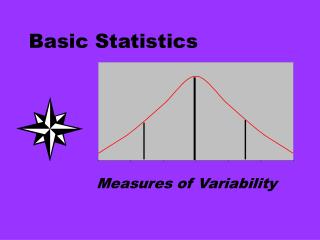
Variability • Measures of variability describe the extent of similarity or difference in a set of scores • These measures include the range, standard deviation, and variance
Standard Deviation (SD) • Standard Deviation – a measure of the variability, or spread, of a set of scores around the mean • Intuitively, the sum of the differences between each score and the mean (known as deviationscores) appears to be a good approach for measuring variability around the mean
SD • Symbolically, we can write this as • Let’s use the scores 1, 2, 6, 6, and 15, where
SD • Now let’s calculate the sum of the deviation scores: = (1-6) + (2-6) + (6-6) + (6-6) + (15-6) = (-5) + (-4) + (0) + (0) + (9) = = -9 + 9 = 0
SD • We can avoid this problem (deviation scores sum to 0) by squaring each deviation score before summing them • This would be written symbolically as
SD • Substituting our X scores again, = (1-6)2 + (2-6)2 + (6-6)2 + (6-6)2 + (15-6)2 = (-5)2 + (-4)2 + (0)2 + (0)2 + (9)2 = 25 + 16 + 0 + 0 + 81 = 122
SD • We then divide this value by n-1 to arrive at the mean squared deviation 122/4 = 30.5 • We then take the square root of this value to bring the units back to the raw score units
Subj Score (x) Deviation (x)2 1 216 22.7 515.29 2 144 -49.3 2430.49 3 183 -10.3 106.09 4 138 -55.3 3058.09 5 212 18.7 349.69 6 180 -13.3 176.89 7 200 6.7 44.89 8 264 70.7 4998.49 9 203 9.7 94.09 =1740 =0 =11774.01 Example calculation of variance and standard deviation on strength scores.
Calculating the SD Using SPSS • Analyze -> Descriptive Statistics -> Frequencies command may be used to determine the standard deviation (you will need to select the “Statistics…” button to choose the “Std. deviation”
Variance • The variance is the square of the standard deviation • It is used most commonly with more advanced statistical procedures such as regression analysis, analysis of variance (ANOVA), and the determination of the reliability of a test
Variance • The variance is also known as the mean square (MS)
Range • The range is equal to the high score minus the low score in a distribution • It is considered an unstable measure of variability, and can change drastically if extreme scores are introduced to the distribution
Range • As a result of gas analysis in a respirometer, an investigator obtains the following four readings of oxygen percentages: 14.9, 10.8, 12.3, and 23.3 • What is the range?
Calculating the Range Using SPSS • Analyze -> Descriptive Statistics -> Frequencies command may be used to calculate the range (you will need to select the “Statistics…” button to choose “Minimum,” “Maximum,” and “Range”
Confidence Intervals Provide an expected upper and lower limit for a statistic at a specified probability level (usually 95% or 99%) CI is dependent upon the sample size, homogeneity of values within the sample and the level of confidence selected by the researcher
Confidence Interval, cont’d For example, a sample mean is an estimate of the population mean A confidence interval provides a band within which the population mean is likely to fall CI = mean ± (standard error × confidence level) The standard error(sM) is the variability of the sampling distribution of the statistic
Calculating a CI Example: n = 30, M = 40, s = 8 CI = 40 ± (1.46 × 2.045) CI = 40 ± 2.99 = 37.01 to 42.99 The value “1.46” came from the following formula: The value “2.045” came from table A.5 (next slide)
Correlation • Correlation “indicates the extent to which two variables are related or associated • The extent to which the direction and size of deviations from the mean in one variable are related to the direction and size of deviations from the mean in another variable”
Categories of Statistical Tests • Parametric • Normal distribution • Equal variances • Independent observations • Nonparametric (distribution free) • Distribution is not normal • Normal curve • Skewness • Kurtosis
Statistics • What statistical techniques tell us • Reliability (significance) of effect • Strength of the relationship (meaningfulness) • Types of statistical techniques • Relationships among variability • Differences among groups • Cause and effect • Correlation is no proof of causation