Download
1 / 37
410 likes | 657 Views
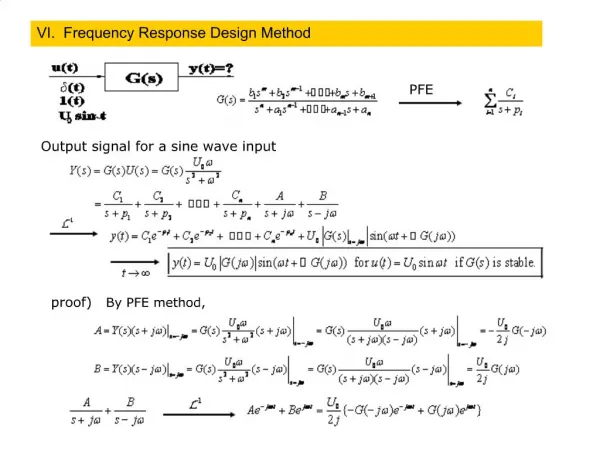
INC341 Frequency Response Method (continue). Lecture 12. Knowledge Before Studying Nyquist Criterion. unstable if there is any pole on RHP (right half plane). Open-loop system:. Characteristic equation:. poles of G(s)H(s) and 1+ G(s)H(s) are the same. Closed-loop system:.

E N D
INC341Frequency Response Method(continue) Lecture 12
Knowledge BeforeStudying Nyquist Criterion unstable if there is anypole on RHP (right half plane)
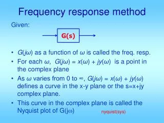
Open-loop system: Characteristic equation: poles ofG(s)H(s) and1+G(s)H(s) are the same Closed-loop system: zero of1+G(s)H(s) ispole ofT(s)
Zero – 1,2,3,4 Poles – 5,6,7,8 Zero – a,b,c,d Poles – 5,6,7,8 Zero – ?,?,?,? Poles – a,b,c,d To know stability, we have to know a,b,c,d
Stability from Nyquist plot From a Nyquist plot, we can tell a number of closed-loop poles on the right half plane. • If there is any closed-loop pole on the right half plane, the system goes unstable. • If there is no closed-loop pole on the right half plane, the system is stable.
Nyquist Criterion Nyquist plot is a plot used to verify stability of the system. mapping contour function mapping all points (contour) from one plane to another by function F(s).
Pole/zero inside the contour has 360 deg. angular change. • Pole/zero outside contour has 0 deg. angular change. • Move clockwise around contour, zero inside yields rotation in clockwise, pole inside yields rotation in counterclockwise
Characteristic equation N = P-Z N = # of counterclockwise direction about the origin P = # of poles of characteristic equation inside contour = # of poles of open-loop system z = # of zeros of characteristic equation inside contour = # of poles of closed-loop system Z = P-N
Characteristic equation • Increase size of the contour to cover the right half plane • More convenient to consider the open-loop system (with known pole/zero)
‘Open-loop system’ Nyquist diagram of Mapping from characteristic equ. to open-loop system by shifting to the left one step Z = P-N Z = # of closed-loop poles inside the right half plane P = # of open-loop poles inside the right half plane N = # of counterclockwise revolutions around -1
Properties of Nyquist plot If there is a gain, K, in front of open-loop transfer function, the Nyquist plot will expand by a factor of K.
Nyquist plot example • Open loop system has pole at 2 • Closed-loop system has pole at 1 • If we multiply the open-loop with a gain, K, then we can move the closed-loop pole’s position to the left-half plane
Nyquist plot example (cont.) • New look of open-loop system: • Corresponding closed-loop system: • Evaluate value of K for stability
Adjusting an open-loop gain to guarantee stability Step I: sketch a Nyquist Diagram Step II: find a range ofK that makes the systemstable!
How to make a Nyquist plot? Easy way by Matlab • Nyquist: ‘nyquist’ • Bode: ‘bode’
Step I: make a Nyquist plot • Starts from an open-loop transfer function (set K=1) • Set and find frequency response • At dc, • Find at which the imaginary part equals zero
Need the imaginary term = 0, Substitute back in to the transfer function And get
At dc, s=0, At imaginary part=0
Step II: satisfying stability condition • P = 2, N has to be 2 to guarantee stability • Marginally stable if the plot intersects -1 • For stability, 1.33K has to be greater than 1 K > 1/1.33 or K > 0.75
Example Evaluate arange ofK that makes the systemstable
Step I: find frequency at which imaginary part = 0 Set the imaginary part = 0 At Plug back in the transfer function and get G = -0.05
Step II: consider stability condition • P = 0, N has to be 0 to guarantee stability • Marginally stable if the plot intersects -1 • For stability, 0.05K has to be less than 1 K < 1/0.05 or K < 20
Gain Margin and Phase Margin Gain margin is the change in open-loop gain (in dB), required at 180 of phase shift to make the closed-loop system unstable. Phase margin is the change in open-loop phase shift, required at unity gain to make the closed-loop system unstable. GM/PM tells how much system can tolerate before going unstable!!!
GM and PM via Bode Plot • The frequency at which the phase equals 180 degrees is called the phase crossover frequency • The frequency at which the magnitude equals 1 is called the gain crossover frequency gain crossover frequency phase crossover frequency
Example Find Bode Plot and evaluate a value ofK that makes the system stable The system has a unity feedback with an open-loop transfer function First, let’s find Bode Plot ofG(s) by assuming that K=40(the value at which magnitude plot startsfrom 0 dB)
GM>0, system is stable!!! • Can increasegain up20 dB without causing instability (20dB = 10) • Start from K = 40 • withK < 400, system is stable
Closed-loop transient and closed-loop frequency responses‘2nd system’
Damping ratio and closed-loop frequency response Magnitude Plot of closed-loop system
Response speed and closed-loop frequency response = frequency at whichmagnitude is3dB down from value at dc (0 rad/sec), or .
Find from Open-loop Frequency Response Nichols Charts From open-loop frequency response, we can find at the open-loop frequency that the magnitude lies between -6dB to-7.5dB (phase between-135to-225)
Relationship betweendamping ratio and phase marginof open-loop frequency response Phase margin ofopen-loop frequency response Can be written in terms ofdamping ratio as following
= 3.7 Example Open-loop system with a unity feedback has a bode plot below, approximate settling time and peak time PM=35