Download
1 / 38
390 likes | 428 Views
This study compares various discretization methods for converting continuous features into discrete ones for machine learning applications. Methods include global vs local, supervised vs unsupervised approaches. Experimental results show improved accuracy with entropy-based discretization.

E N D
Discretization of continuous attributes CS583 Spring 2005 Yi Zhang Peng Fan
Outline • Introduction • Three discretization methods comparison • Experimental Results • Related Work • Summary
Introduction • A discretization algorithm converts continuous features into discrete features. A good discretization algorithm should not increase the error rate much
Age [5,15] Age [16,24] Age [25,67] Discretization • Divide the range of a continuous (numeric) attribute into intervals • Store only the interval labels • Important for association rules and classification
Motivation • Some algorithms are limited to discrete inputs • Many algorithms discretize as part of the learning algorithm(Decision Tree), could this part be improved? • Efficiency. Continuous features drastically slows the learning algorithms
Classifying Discretization Algorithms Discretization can be classified into two dimensions: • Supervised vs. Unsupervised • Global vs. Local
Supervised vs. Unsupervised Make use of class label • Supervised algorithms: • Entropy-based [Fayyad & Irani 93 and others] • Binning [Holte 93] • Unsupervised algorithms: • Equal width intervals • Equal frequency intervals
Global vs. Local • Global methods(Binning) produce a mesh over the entire n-dimensional continuous instance space • Local methods(Decision tree) produce partitions that are applied to localized region of the instance space.
Equal Interval Width (Binning) • Given the # of k, divide the training-set range into k equal-sized bins • Problems: • Where dose k come from? • Sensitive to outliers
Holte’s OneR Sort the training examples in increasing order according to the value of the numeric attribute values of temperature: 64 65 68 69 70 71 72 72 75 75 80 81 83 85 Y N Y Y Y N N Y Y Y N Y Y N
Holte’s OneR • Place breakpoints in the sequence whenever the class changes Split on 72 – 2 different classes! Easy fix: move the breakpoint to 73.5 producing a mixed partitioning with “no” as majority class • Take the majority class for each partition
Holte’s OneR • Since it may lead to one bin for only one value constrain to forms bins of at least some minimum size MIN_INST() • Holte’s empirical analysis Min = 6
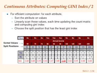
Entropy-based Partitioning • Intuitively, find the best split so that the bins are as pure as possible. • Information split: I(S1,S2) = (|S1|/|S|) Entropy(S1)+ (|S2|/|S|) Entropy(S2) • Information gain of the split: Gain(v,S) = Entropy(S) – I(S1,S2) Goal: split with maximal information gain • Process is recursively applied to partitions obtained until some stopping criterion is met creating multiple intervals • This is a supervised method.
Experimental Setup • Compare equal-width (k=10 & K=2*logL), Holte’s 1R(Min=6), and entropy-based. • Compared C4.5 & Naïve-bayes with and without the filter discretizations. • Choose 16 datasets from UCI, all containing at least on continuous feature.
Accuracies using Naive-Bayes with different discretization methods
Result for C4.5 accuracy difference of pre-discretized data minus original C4.5
Result for Naïve-Bayes accuracy difference of pre-discretized data minus original Naïve-Bayes
Conclusions • The average performance of the entropy-discretized NB is 83.97% Original NB is 76.57% C4.5 is 83.26% Original C4.5 is 82.25% • The supervised learning methods are slightly better • The global entropy-based method seems to be the best choice here
Chi-square based methods • In discretization problem, a compromise must be found between information quality and statistical quality: • Information quality: Homogeneous intervals in regard to the attribute to predict. • Statistical quality: Sufficient sample size in every interval to ensure generalization. • Entropy-based criteria focus on the information quality, while chi-square criteria focus on the statistical quality. • Examples: • ChiSplit top-down, local • ChiMerge bottom-up, local • Khiops top-down, global
Chi-Square Calculation • Χ2 (chi-square) test • Two main use of chi-square test: • Test independence of two factors: the larger the Χ2 value, the more likely the factors are related • Test similarity of two distributions: the smaller the Χ2 value, the more likely the two distributions are similar
Chi-Square Calculation: An Example Exp(S,A) = 45 * 30 / 150 = 9 ; Exp(S,B) = 45 * 120 / 150 = 36 9 36 21 84 It shows that like_science_fiction and play_computer_game are correlated in the group
ChiSplit(Bertier&Bouroche) • Top-down approach. • It searches for the best split of an interval, by maximizing the chi-square criterion applied to the two sub-intervals adjacent to the splitting point: the interval is split if both sub-intervals substantially differ statistically. • Stopping rule: user-defined chi-square threshold .
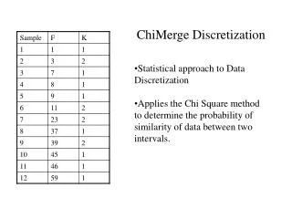
ChiMerge (Kerber 1991) • Initialization step • Place each distinct continuous value into its own interval • Bottom-up fashion • Using chi-square test determine when adjacent intervals should be merged • Repeat until a stopping criteria (set manually) is met
Chi-Merge Example 1 2 1 2 0.5 2.5 0.5 2.5 In this case, 17.92 will emerge with 16.92, instead of 18.08
Iterative Discretization (Pazzani&M.J.) • Initially, form a set of intervals using Equal Width Discretization or Entropy-based Method. • Iteratively adjust the intervals to minimize naïve-Bayesian classifiers’ classification error on the training data. • Two adjustment operations: merging or splitting. • Very time-assuming when data are large.
Proportional k-Interval Discretization (Yang&Webb) • Discretization bias and variance: • Bias: errors result from our algorithms. • Variance: errors result from random variation in the training data and random behavior of the algorithms. • Bias and variance trade-off: (when training data are fixed)
Proportional k-Interval Discretization (Contd.) • For N training instances • s*t=N, s=t. (s: desired interval size; t: # of intervals) • Discretize it into sqrt(N) intervals, with sqrt(N) instances in each interval. • Advantage • When N increase, both bias and variance decrease!
Weighted Proportional k-Interval Discretization (Yang&Webb) • When N is small Proportional k-Interval Discretization tends to produce small intervals resulting in high variance. • Ensure a minimum interval size to prevent high variance: • s*t=N, s-m=t. (s: desired interval size; t: # of intervals; m=30)
Atomic interval Non-Disjoint Discretization (Yang&Webb) • In Naïve-Bayesian classification, we have the following estimation after discretization: • When is near either boundary of (a,b], the right side is less likely to provide relevant information about . interval
Experimental Validation • Discretization algorithms: • Equal Width Discretization, Equal Frequency Discretization, Entropy Minimization Discretization, Proportional K-Interval Discretization, Lazy Discretization, Non-Disjoint Discretization, and Weighted Proportional K-Interval Discretization. • Classification algorithm: Naïve-Bayesian. • Results: LD,NDD and WPKD performs better, but LD can’t scale to large data.
Combine NDD and WPKID? • Weighted Non-Disjoint Discretization • Interval size produced by WPKID. • Combining three atomic intervals into one interval.
References • Supervised and Unsupervised Discretization of Continuous Features (Dougherty,Kohavi&Sahami) • Chimerge : Discretization of numeric attributes (Kerber) • Khiops: A Statistical Discretization Method of Continuous Attributes (Boulle) • Analyse des donn´ees multidimensionnelles (Bertier&Bouroche) • An iterative improvement approach for the discretization of numeric attributes in Bayesian classifiers (Pazzani&J.) • Proportional K-Interval Discretization for naïve-Bayes Classifiers (Yang&Webb) • Weighted Proportional K-Interval Discretization for naïve-Bayes Classifiers (Yang&Webb) • Non-Disjoint Discretization for naïve-Bayes Classifiers (Yang&Webb) • A Comparative Study of Discretization Mehods for Naïve-Bayes Classifiers (Yang&Webb)