Download
1 / 38
380 likes | 390 Views
Discretization for PDEs. Chunfang Chen ,Danny Thorne Adam Zornes, Deng Li CS 521 Feb., 9,2006. Classification of PDEs. Different mathematical and physical behaviors: Elliptic Type Parabolic Type Hyperbolic Type System of coupled equations for several variables:

E N D
Discretization for PDEs Chunfang Chen ,Danny Thorne Adam Zornes, Deng Li CS 521 Feb., 9,2006
Classification of PDEs Different mathematical and physical behaviors: • Elliptic Type • Parabolic Type • Hyperbolic Type System of coupled equations for several variables: • Time : first-derivative (second-derivative for wave equation) • Space: first- and second-derivatives
Classification of PDEs (cont.) General form of second-order PDEs ( 2 variables)
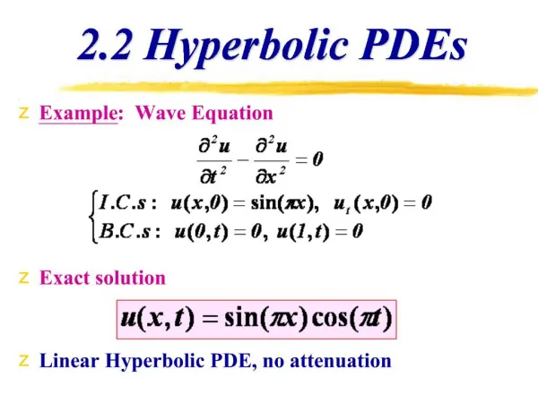
PDE Model Problems • Hyperbolic (Propagation) • Advection equation (First-order linear) • Wave equation (Second-order linear)
PDE Model Problems (cont.) • Parabolic (Time- or space-marching) • Burger’s equation(Second-order nonlinear) • Fourier equation (Second-order linear) (Diffusion / dispersion)
PDE Model Problems (cont.) • Elliptic (Diffusion, equilibrium problems) • Laplace/Poisson (second-order linear) • Helmholtz equation (second-order linear)
PDE Model Problems (cont.) • System of Coupled PDEs • Navier-Stokes Equations
Well-Posed Problem Numerically well-posed • Discretization equations • Auxiliary conditions (discretized approximated) • the computational solution exists (existence) • the computational solution is unique (uniqueness) • the computational solution depends continuously on the approximate auxiliary data • the algorithm should be well-posed (stable) also
Boundary and InitialConditions R • Initial conditions:starting point for propagation problems • Boundary conditions:specified on domain boundaries to provide the interior solution in computational domain R s n
Numerical Methods • Complex geometry • Complex equations (nonlinear, coupled) • Complex initial / boundary conditions • No analytic solutions • Numerical methods needed !!
Numerical Methods Objective: Speed, Accuracy at minimum cost • Numerical Accuracy(error analysis) • Numerical Stability(stability analysis) • Numerical Efficiency (minimize cost) • Validation (model/prototype data, field data, analytic solution, theory, asymptotic solution) • Reliability and Flexibility(reduce preparation and debugging time) • Flow Visualization(graphics and animations)
computational solution procedures Governing Equations ICS/BCS System of Algebraic Equations Equation (Matrix) Solver ApproximateSolution Discretization Ui (x,y,z,t) p (x,y,z,t) T (x,y,z,t) or (,,, ) Continuous Solutions Finite-Difference Finite-Volume Finite-Element Spectral Boundary Element Hybrid Discrete Nodal Values Tridiagonal ADI SOR Gauss-Seidel Krylov Multigrid DAE
Discretization • Time derivatives almost exclusively by finite-difference methods • Spatial derivatives - Finite-difference: Taylor-series expansion - Finite-element: low-order shape function and interpolation function, continuous within each element - Finite-volume: integral form of PDE in each control volume - There are also other methods, e.g. collocation, spectral method, spectral element, panel method, boundary element method
Finite Difference • Taylor series • Truncation error • How to reduce truncation errors? • Reduce grid spacing, use smaller x = x-xo • Increase order of accuracy, use larger n
Finite Difference Scheme • Forward difference • Backward difference • Central difference
y x Example : Poisson Equation (-1,1) (1,1) (-1,-1) (1,-1)
Rectangular Grid After we discretize the Poisson equation on a rectangular domain, we are left with a finite number of gird points. The boundary values of the equation are the only known grid points
What to solve? Discretization produces a linear system of equations. The A matrix is a pentadiagonal banded matrix of a standard form: A solution method is to be performed for solving
Matrix Storage We could try and take advantage of the banded nature of the system, but a more general solution is the adoption of a sparse matrix storage strategy.
Limitations of Finite Differences • Unfortunately, it is not easy to use finite differences in complex geometries. • While it is possible to formulate curvilinear finite difference methods, the resulting equations are usually pretty nasty.
Finite Element Method • The finite element method, while more complicated than finite difference methods, easily extends to complex geometries. • A simple (and short) description of the finite element method is not easy to give. Weak Form Matrix System PDE
Finite Element Method (Variational Formulations) • Find u in test space H such that a(u,v) = f(v) for all v in H, where a is a bilinear form and f is a linear functional. • V(x,y) = j Vjj(x,y), j = 1,…,n • I(V) = .5 j j AijViVj - j biVi, i,j = 1,…,n • Aij = a( j, j), i = 1,…,n • Bi = f j, i = 1,…,n • The coefficients Vj are computed and the function V(x,y) is evaluated anyplace that a value is needed. • The basis functions should have local support (i.e., have a limited area where they are nonzero).
Time Stepping Methods • Standard methods are common: • Forward Euler (explicit) • Backward Euler (implicit) • Crank-Nicolson (implicit) θ = 0, Fully-Explicit θ = 1, Fully-Implicit θ = ½, Crank-Nicolson
Time Stepping Methods (cont.) • Variable length time stepping • Most common in Method of Lines (MOL) codes or Differential Algebraic Equation (DAE) solvers
Solving the System • The system may be solved using simple iterative methods - Jacobi, Gauss-Seidel, SOR, etc. • Some advantages: - No explicit storage of the matrix is required - The methods are fairly robust and reliable • Some disadvantages - Really slow (Gauss-Seidel) - Really slow (Jacobi)
Solving the System • Advanced iterative methods (CG, GMRES) CG is a much more powerful way to solve the problem. • Some advantages: • Easy to program (compared to other advanced methods) • Fast (theoretical convergence in N steps for an N by N system) • Some disadvantages: • Explicit representation of the matrix is probably necessary • Applies only to SPD matrices
Multigrid Algorithm: Components • Residual • compute the error of the approximation • Iterative method/Smoothing Operator • Gauss-Seidel iteration • Restriction • obtain a ‘coarse grid’ • Prolongation • from the ‘coarse grid’ back to the original grid
Residual Vector • The equation we are to solve is defined as: • So then the residual is defined to be: • Where uq is a vector approximation for u • As the u approximation becomes better, the components of the residual vector(r) , move toward zero
Multigrid Algorithm: Components • Residual • compute the error of your approximation • Iterative method/Smoothing Operator • Gauss-Seidel iteration • Restriction • obtain a ‘coarse grid’ • Prolongation • from the ‘coarse grid’ back to the original grid
Multigrid Algorithm: Components • Residual • compute the error of your approximation • Iterative method/Smoothing Operator • Gauss-Seidel iteration • Restriction • obtain a ‘coarse grid’ • Prolongation • from the ‘coarse grid’ back to the original grid
The Restriction Operator • Defined as ‘half-weighted’ restriction. • Each new point in the courser grid, is dependent upon it’s neighboring points from the fine grid
Multigrid Algorithm: Components • Residual • compute the error of your approximation • Iterative method/Smoothing Operator • Gauss-Seidel iteration • Restriction • obtain a ‘coarse grid’ • Prolongation • from the ‘coarse grid’ back to the original grid
The Prolongation Operator • The grid change is exactly the opposite of restriction
Prolongation vs. Restriction • The most efficient multigrid algorithms use prolongation and restriction operators that are directly related to each other. In the one dimensional case, the relation between prolongation and restriction is as follows:
Full Multigrid Algorithm 1.Smooth initial U vector to receive a new approximation Uq 2.Form residual vector: Rq =b -A Uq 3. Restrict Rq to the next courser grid Rq-1 4. Smooth Ae= Rq-1 starting with e=0 to obtain eq-1 5.Form a new residual vector using: Rq-1= Rq-1 -A eq-1 6. Restrict R2 (5x? where ?5) down to R1(3x? where ?3) 7. Solve exactly for Ae= R1 to obtain e1 8. Prolongate e1e2 & add to e2 you got from restriction 9. Smooth Ae= R2 using e2 to obtain a new e2 10. Prolongate eq-1 to eq and add to Uq
Reference • http://www.mgnet.org/~douglas/ • http://www.mgnet.org/~douglas/Classes/cs521/2006-index.html
Practice (Option) Introduce the following processing by read the book “A Tutorial on Elliptic PDE Solvers and Their Parallelization” Weak Form Discrete Matrix PDE