Download
1 / 48
480 likes | 537 Views
Understand the importance, process, and advantages of discretization in data analytics. Learn about various perspectives, steps, properties, and taxonomy of discretization methods for effective data handling.

E N D
Discretization • Introduction • Perspectives and Background • Properties and Taxonomy • Experimental Comparative Analysis
Discretization • Introduction • Perspectives and Background • Properties and Taxonomy • Experimental Comparative Analysis
Introduction • Data usually comes in different formats, such as discrete, numerical, continuous, categorical, etc. • Numerical data, assumes that the data is ordinal, there is an order among the values. However, in categorical data, no order can be assumed. • If data is continuous, there is a need to discretize the features for some learners.
Introduction • The discretization process transforms quantitative data into qualitative data, that is, numerical attributes into discrete or nominal attributes with a finite number of intervals, obtaining a non-overlapping partition of a continuous domain. • In practice, discretization can be viewed as a data reduction method since it maps data from a huge spectrum of numeric values to a greatly reduced subset of discrete values.
Introduction • In supervised learning, and specifically classification, we can define the discretization as follows: Assuming a data set consisting of N examples and C target classes, a discretization algorithm would discretize the continuous attribute A in this data set into m intervals D = {[d0, d1], (d1, d2], …, (dm−1, dm]}, where d0 is the minimal value, dm is the maximal value and di < di+i, for i = 0, 1, ...,m−1. Such a discrete result D is called a discretization scheme on attribute A and P = {d1, d2, ..., dm−1} is the set of cut points of attribute A.
Introduction • Advantages of using discretization: • Many DM algorithms are primarily oriented to handle nominal attributes. • The reduction and the simplification of data. • Compact and shorter results. • For both researchers and practitioners, discrete attributes are easier to understand, use, and explain. • Negative effect: loss of information.
Discretization • Introduction • Perspectives and Background • Properties and Taxonomy • Experimental Comparative Analysis
Perspectives and Background • Important concepts: • Features. • Instances. • Cut Point. Real value that divides the range into two adjacent intervals. • Arity. Number of partitions or intervals. For example, if the arity of a feature after being discretized is m, then there will be m−1 cut points.
Perspectives and Background Typical discretization process:
Perspectives and Background • Discretization steps: • Sorting. The continuous values for a feature are sorted in either descending or ascending order. Sorting must be done only once and for all the start of discretization. • Selection of a Cut Point. The best cut point or the best pair of adjacent intervals should be found in the attribute range in order to split or merge in a following required step. An evaluation measure or function is used to determine the correlation, gain or improvement in performance.
Perspectives and Background • Discretization steps: • Splitting/Merging. For splitting all the possible cut points from the whole universe within an attribute must be evaluated. The universe is formed from all the different real values presented in an attribute. For merging, the discretizer aims to find the best adjacent intervals to merge in each iteration. • Stopping Criteria. When to stop the discretization process.
Perspectives and Background • Related and Advanced Works: • Discretization Specific Analysis. • Optimal Multisplitting. • Discretization of Continuous Labels. • Fuzzy Discretization. • Cost-Sensitive Discretization. • Semi-Supervised Discretization.
Discretization • Introduction • Perspectives and Background • Properties and Taxonomy • Experimental Comparative Analysis
Properties and Taxonomy • Common properties: • Main characteristics of a discretizer. • Static vs. Dynamic. Moment and independence which the discretizer operates in relation to the learner. A dynamic discretizer acts when the learner is building the model. a static discretizer proceeds prior to the learning task and it is independent from the learner. • Univariate vs. Multivariate. Multivariate techniques simultaneously consider all attributes to define the initial set of cut points or to decide the best cut point altogether. Univariate discretizers only work with a single attribute at a time.
Properties and Taxonomy • Common properties: • Main characteristics of a discretizer. • Supervised vs. Unsupervised. Unsupervised discretizers do not consider the class label whereas supervised ones do. Most discretizers proposed in the literature are supervised. • Splitting vs. Merging. Procedure used to create or define new intervals. Splitting methods establish a cut point among all the possible boundary points and divide the domain into two intervals. Merging methods start with a pre-defined partition and remove a candidate cut point to mix both adjacent intervals.
Properties and Taxonomy • Common properties: • Main characteristics of a discretizer. • Global vs. Local. To make a decision, a discretizer can either require all available data in the attribute or use only partial information. A discretizer is said to be local when it only makes the partition decision based on local information. • Direct vs. Incremental. Direct discretizers divide the range into k intervals simultaneously. incremental methods begin with a simple discretization and pass through an improvement process, requiring an additional criterion to know when to stop it.
Properties and Taxonomy • Common properties: • Main characteristics of a discretizer. • Evaluation Measure. • Information: Entropy, Gini index. • Statistical: Dependency, correlation, probability, bayesian properties, contingeny coefficients. • Rough Sets: Lower and upper approximations, class separability. • Wrapper: Error provided by a learner. • Binning: No evaluation measure.
Properties and Taxonomy • Common properties: • Other properties. • Parametric vs. Non-Parametric. Automatic determination of the number of intervals for each attribute by the discretizer. • Top Down vs. Bottom-Up. Similar to splitting vs. Merging. • Stopping condition. Mechanism used to stop the discretization process and must be specified in nonparametric approaches.
Properties and Taxonomy • Common properties: • Other properties. • Disjoint vs. Non-Disjoint. Disjoint methods discretize the value range of the attribute into disassociated intervals, without overlapping, whereas non-disjoint methods dicsretize the value range into intervals that can overlap. • Ordinal vs. Nominal. Ordinal discretization transforms quantitative data into ordinal qualitative data whereas nominal discretization transforms it into nominal qualitative data, discarding the information about order.
Properties and Taxonomy • Common properties: • Criteria to compare discretization methods. • Number of Intervals. • Inconsistency. • Predictive Classification Rate. • Time requirements
Properties and Taxonomy Discretization Methods (1):
Properties and Taxonomy Discretization Methods (2):
Properties and Taxonomy Discretization Methods (3):
Properties and Taxonomy Discretization Methods (4):
Properties and Taxonomy Taxonomy
Properties and Taxonomy Taxonomy
Description of Representative Methods Splitting
Description of Representative Methods Splitting Equal Width or Frequency — In equal width, the continuous range of a feature is divided into intervals that have an equal width and each interval represents a bin. The arity can be calculated by the relationship between the chosen width for each interval and the total length of the attribute range. In equal frequency, an equal number of continuous values are placed in each bin. Thus, the width of each interval is computed by dividing the length of the attribute range by the desired arity.
Description of Representative Methods Splitting MDLP — This discretizer uses the entropy measure to evaluate candidate cut points. Entropy is one of the most commonly used discretization measures in the literature. The entropy of a sample variable X is where x represents a value of X and px its estimated probability of occurring. It corresponds to the average amount of information per event where information of an event is defines as:
Description of Representative Methods Splitting MDLP — Information is high for lower probable events and low otherwise. This discretizer uses the Information Gain of a cut point, which is defined as where A is the attribute in question, T is a candidate cut point and S is the set of N examples. So, Si is a partitioned subset of examples produced by T. The MDLP discretizer applies the Minimum Description Length Principle to decide the acceptation or rejection for each cut point and to govern the stopping criterion.
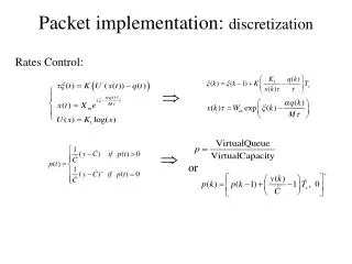
Description of Representative Methods Splitting PKID — When discretizing a continuous attribute for which there are N instances, supposing that the desired interval frequency is s and the desired interval number is t, PKID calculates s and t by the following expressions: Thus, this discretizer is an equal frequency (or equal width) discretizer where both the interval frequency and number of intervals have the same quantity and they only depend on the number of instances in training data.
Description of Representative Methods Splitting FFD — Stands for fixed frequency discretization and was proposed for managing bias and variance especially in naive-bayes based classifiers. To discretize a continuous attribute, FFD sets a sufficient interval frequency, f. Then it discretizes the ascendingly sorted values into intervals of frequency f.Thus each interval has approximately the same number f of training instances with adjacent values.
Description of Representative Methods Splitting CAIM — Stands for Class-Attribute Interdependency Maximization criterion, which measures the dependency between the class variable C and the discretized variable D for attibute A. The method requires the computation of the quanta matrix, which, in summary, collects a snapshot of the number of real values of A within each interval and for each class of the corresponding example. The criterion is calculated as:
Description of Representative Methods Merging ChiMerge — χ2 is a statistical measure that conducts a significance test on the relationship between the values of an attribute and the class. This statistic determines the similarity of adjacent intervals based on some significance level. Actually, it tests the hypothesis that two adjacent intervals of an attribute are independent of the class. χ2 is computed as:
Description of Representative Methods Merging ChiMerge — It is a supervised, bottom-up discretizer. At the beginning, each distinct value of the attribute is considered to be one interval. χ2 tests are performed for every pair of adjacent intervals. Those adjacent intervals with the least χ2 value are merged until the chosen stopping criterion is satisfied.
Description of Representative Methods Merging Chi2 — It can be explained as an automated version of ChiMerge. Here, the statistical significance level keeps changing to merge more and more adjacent intervals as long as an inconsistency criterion is satisfied. We understand inconsistency to be two instances that match but belong to different classes. Like ChiMerge, χ2 statistic is used to discretize the continuous attributes until some inconsistencies are found in the data. The stopping criterion is achieved when there are inconsistencies in the data considering a limit of zero or δ inconsistency level as default.
Description of Representative Methods Merging • Modified Chi2 — In the original Chi2 algorithm, the stopping criterionwas defined as the point at which the inconsistency rate exceeded a predefined rate δ. The δ value could be given after some tests on the training data for different data sets. The modification proposed was to use the level of consistency checking coined from Rough Sets Theory. Thus, this level of consistency replaces the basic inconsistency checking, ensuring that the fidelity of the training data could be maintained to be the same after discretization and making the process completely automatic.
Description of Representative Methods Merging FUSINTER — This method uses the same strategy as the ChiMerge method, but rather than trying to merge adjacent intervals locally, FUSINTER tries to find the partition which optimizes the measure. Next, we provide a short description: • Obtain the boundary cut points after an increasing sorting of the values and the formation of intervals with run of examples of the same class. • Construct a matrix with a similar structure like a quanta matrix. • Find two adjacent intervals whose merging would improve the value of the criterion and check if they can be merged using a differential criterion. • Repeat until no improvement is possible.
Discretization • Introduction • Perspectives and Background • Properties and Taxonomy • Experimental Comparative Analysis
Experimental Comparative Analysis Framework 10-FCV. Parameters recommended by the authors of the algorithms. 6 classifiers: C4.5, DataSqueezer, KNN, Naïve Bayes, PUBLIC, Ripper. 30 discretizers. 40 data sets. Accuracy and Kappa, number of intervals and inconsistency as evaluation measures.
Experimental Comparative Analysis Best Results: Number of Intervals, Inconsistency
Experimental Comparative Analysis Best Results: Accuracy
Experimental Comparative Analysis Best Results: Kappa
Experimental Comparative Analysis Results achieved (1) • Heter-Disc, MVD and Distance are the best discretizers in terms of number of intervals. • The inconsistency rate both in training data and test data follows a similar trend for all discretizers. • In decision trees (C4.5 and PUBLIC), a subset of discretizers can be stressed as the best performing ones. Considering average accuracy, FUSINTER, ChiMerge and CAIM stand out from the rest. Considering average kappa, Zeta and MDLP are also added to this subset.
Experimental Comparative Analysis Results achieved (2) • Considering rule induction (DataSqueezer and Ripper), the best performing discretizers are Distance, Modified Chi2, Chi2, PKID andMODL in average accuracy and CACC, Ameva,CAIM and FUSINTER in average kappa. • With respect to lazy and bayesian learning, KNN and Naïve Bayes, the subset of remarkable discretizers is formed by PKID,FFD, Modified Chi2, FUSINTER, ChiMerge, CAIM, EqualWidth and Zeta, when average accuracy is used; and Chi2, Khiops, EqualFrequency and MODL must be added when average kappa is considered.
Experimental Comparative Analysis Resultsachieved (3) • Wecan stress a subset of global bestdiscretizersconsidering a trade-off betweenthenumber of intervals and accuracyobtained. • In thissubset, wecan includeFUSINTER, Distance, Chi2, MDLP and UCPD.