Download
1 / 19
210 likes | 419 Views
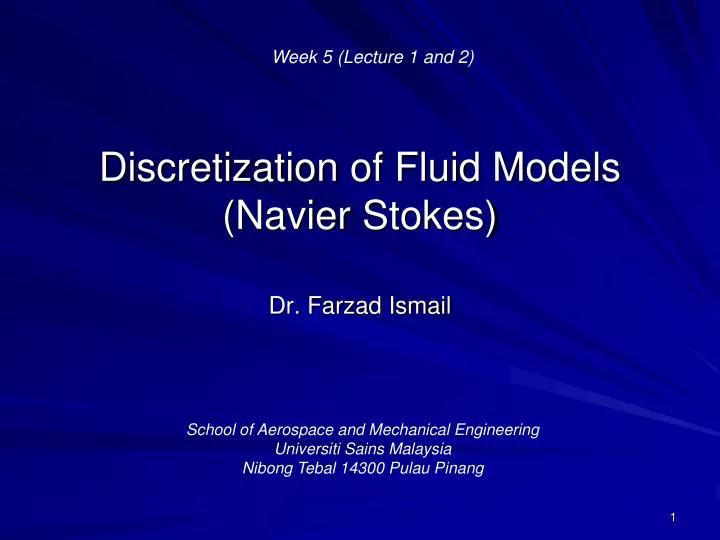
Week 5 (Lecture 1 and 2). Discretization of Fluid Models ( Navier Stokes). Dr. Farzad Ismail. School of Aerospace and Mechanical Engineering Universiti Sains Malaysia Nibong Tebal 14300 Pulau Pinang. Preview. We have talked about various schemes to solve model problems.

E N D
Week 5(Lecture 1 and 2) Discretization of Fluid Models(Navier Stokes) Dr. Farzad Ismail School of Aerospace and Mechanical Engineering Universiti Sains Malaysia Nibong Tebal 14300 Pulau Pinang
Preview • We have talked about various schemes to solve model problems. • Would like to use the knowledge to solve real fluid models. • Before we do that, first need to understand the mathematical and physical nature of fluid dynamics.
The Compressible Navier Stokes • One of the most complete mathematical models for fluids. • Includes compressibility, viscous, heat transfer, advection, pressure effects. • Can also be used to account for reacting fluids
The Compressible Navier Stokes (cont’d) • In 2D, a system of 4 x 4 (3D - 5 x 5) • A hybrid of hyperbolic and parabolic types for unsteady cases • Elliptic in nature for steady cases • Decompose NS model into inviscid (compressible) and viscous (incompressible) parts
2D Incompressible Navier Stokes (NS) How do you know that mass equation is numerically satisfied?
Pressure Poisson (1) (2) (3) (4) (1) (4) (3)
Pressure Poisson (cont’d) (3) (*) (**) Solve * and ** for incompressible NS
2D Incompressible Navier Stokes (NS) The momentum can be rewritten (***)
Exercise Take the gradient of Eqn (***), apply the mass equation and show that What does this equation provide? More importantly, what is the nature of this eqn And how to solve it?
2D Incompressible NS (cont’d) • Incompressible flow has only mass and momentum equations • The energy equation drops out (3 eqns, 3 unknowns) • Mass is implicitly solved through the pressure-Poisson equation • Pressure-based solver (i.e. SIMPLE, PISO) • Requires iterations to satisfy velocity divergence- expensive! • Adds an elliptic nature to pde on top of the hyperbolic and parabolic natures • Flow is ‘smooth’
Choice of Grid Discretization • It is not critical for unsteady problems but it is crucial for steady-state problems • Elliptic problems have issues with certain errors not being removed even after many iterations. • Collocated: all variables are stored at the same location • Worst choice, since there will be some errors that will never be removed! • Compact: • Better choice, but there will be at least one type of errors that will never be removed! • Staggered- best choice for elliptic problem, but…
Staggered Grid What about p, F,G, H’s?
Initial & Boundary Conditions • For elliptic problems, IC is not so much a big deal • Will just determine how quick solution reach steady-state • But the BC is very critical! • Not only determines the efficiency of the computations • But will also determine what is the final outcome • Unphysical BC may lead to huge problems?Why? • Concept of Ghost Cells • No slip condition along and no outflow/inflow through boundaries
Boundary Conditions (cont’d) • How to compute ghost cells? • Combine BC and the equations of motions to extrapolate the values outside the computational domain • Take horizontal boundary, v=0 (obvious) but u may not be unless wall is not moving (no slip) • Can use mass equation
Boundary Conditions (cont’d) • Nature of u,v at boundaries • v=0 at boundary but u may not be zero; v even function • vy= -ux = 0 (by mass), implies that u is constant along wall and that integrating u wrt x gives u(x,y) as a constant plus a linear Variation along y. • The ghost quantities (previous Fig) via the y-momentum:
Vo and H(y) are zero on the boundary, this simplifies to where vT are expanded from v0 via Taylor series • Since v0=0 and assume that the square of v and the high order terms are negligible, hence
Since v is an even function, • The same can be done for other walls and similar approach for (u,v)
Algorithm for Incompressible NS • Apply the appropriate BC • Solve for the preliminary u*, v* based on (u,v,p) of IC and BC • Compute the Pressure-Poisson equation to solve for p* • Iterate until reach required error tolerance • Check the discrete velocity divergence, if criterion is met, proceed to the next time level. If not go back to step 1 and continue the iteration within the same time-level