Download
1 / 34
660 likes | 2.18k Views
Discrete-time Random Signals . Until now, we have assumed that the signals are deterministic, i.e., each value of a sequence is uniquely determined.

E N D
Discrete-time Random Signals • Until now, we have assumed that the signals are deterministic, i.e., each value of a sequence is uniquely determined. • In many situations, the processes that generate signals are so complex as to make precise description of a signal extremely difficult or undesirable. • A random or stochastic signal is considered to be characterized by a set of probability density functions.
Stochastic Processes • Random (or stochastic) process (or signal) • A random process is an indexed family of random variables characterized by a set of probability distribution function. • A sequence x[n], <n< . Each individual sample x[n] is assumed to be an outcome of some underlying random variableXn. • The difference between a single random variable and a random process is that for a random variable the outcome of a random-sampling experiment is mapped into a number, whereas for a random process the outcome is mapped into a sequence.
Stochastic Processes (continue) • Probability density function of x[n]: • Joint distribution of x[n] and x[m]: • Eg., x1[n] = Ancos(wn+n), where An and nare random variables for all < n < , then x1[n] is a random process.
Independence and Stationary • x[n] and x[m] are independent iff • x is a stationary process iff for all k. • That is, the joint distribution of x[n] and x[m] depends only on the time difference m n.
Stationary (continue) • Particularly, whenm = n for a stationary process: It implies that x[n] is shift invariant.
Stochastic Processes vs. Deterministic Signal • In many of the applications of discrete-time signal processing, random processes serve as models for signals in the sense that a particular signal can be considered a sample sequence of a random process. • Although such a signals are unpredictable – making a deterministic approach to signal representation is inappropriate – certain average properties of the ensemble can be determined, given the probability law of the process.
Expectation • Mean (or average) • denotes the expectation operator • For independent random variables
Mean Square Value and Variance • Mean squared value • Variance
Autocorrelation and Autocovariance • Autocorrelation • Autocovariance
Stationary Process • For a stationary process, the autocorrelation is dependent on the time difference m n. • Thus, for stationary process, we can write • If we denote the time difference by k, we have
Wide-sense Stationary • In many instances, we encounter random processes that are not stationary in the strict sense. • If the following equations hold, we call the process wide-sense stationary (w. s. s.).
Time Averages • For any single sample sequence x[n], define their time average to be • Similarly, time-average autocorrelation is
Ergodic Process • A stationary random process for which time averages equal ensemble averages is called an ergodic process:
Ergodic Process (continue) • It is common to assume that a given sequence is a sample sequence of an ergodic random process, so that averages can be computed from a single sequence. • In practice, we cannot compute with the limits, but instead the quantities. • Similar quantities are often computed as estimates of the mean, variance, and autocorrelation.
Properties of correlation and covariance sequences • Property 1:
Properties of correlation and covariance sequences (continue) • Property 2: • Property 3
Properties of correlation and covariance sequences (continue) • Property 4:
Properties of correlation and covariance sequences (continue) • Property 5: • If
Fourier Transform Representation of Random Signals • Since autocorrelation and autocovariance sequences are all (aperiodic) one-dimensional sequences, there Fourier transform exist and are bounded in |w|. • Let the Fourier transform of the autocorrelation and autocovariance sequences be
Fourier Transform Representation of Random Signals (continue) • Consider the inverse Fourier Transforms:
Fourier Transform Representation of Random Signals (continue) • Consequently, • Denote to be the power density spectrum (or power spectrum) of the random process x.
Power Density Spectrum • The total area under power density in [,] is the total energy of the signal. • Pxx(w) is always real-valued since xx(n) is conjugate symmetric • For real-valued random processes, Pxx(w) = xx(ejw) is both real and even.
Mean and Linear System • Consider a linear system with frequency response h[n]. If x[n] is a stationary random signal with mean mx, then the output y[n] is also a stationary random signal with mean mx equaling to • Since the input is stationary, mx[nk] = mx , and consequently,
Stationary and Linear System • If x[n] is a real and stationary random signal, the autocorrelation function of the output process is • Since x[n] is stationary , {x[nk]x[n+mr] } depends only on the time difference m+kr.
Stationary and Linear System (continue) • Therefore, The output power density is also stationary. • Generally, for a LTI system having a wide-sense stationary input, the output is also wide-sense stationary.
Power Density Spectrum and Linear System • By substituting l = rk, where • A sequence of the form of chh[l] is calleda deterministic autocorrelation sequence.
Power Density Spectrum and Linear System (continue) • A sequence of the form of Chh[l]l = rk, where Chh(ejw) is the Fourier transform of chh[l]. • For realh, • Thus
Power Density Spectrum and Linear System (continue) • We have the relation of the input and the output power spectrums to be the following:
Power Density Property • Key property: The area over a band of frequencies, wa<|w|<wb, is proportional to the power in the signal in that band. • To show this, consider an ideal band-pass filter. Let H(ejw) be the frequency of the ideal band pass filter for the band wa<|w|<wb. • Note that |H(ejw)|2and xx(ejw) are both even functions. Hence,
White Noise (or White Gaussian Noise) • A white noise signal is a signal for which • Hence, its samples at different instants of time are uncorrelated. • The power spectrum of a white noise signal is a constant • The concept of white noise is very useful in quantization error analysis.
White Noise (continue) • The average power of a white-noise is therefore • White noise is also useful in the representation of random signals whose power spectra are not constant with frequency. • A random signal y[n] with power spectrum yy(ejw) can be assumed to be the output of a linear time-invariant system with a white-noise input.
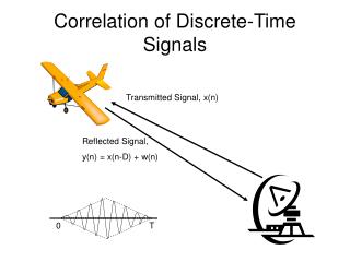
Cross-correlation • The cross-correlation between input and output of a LTI system: • That is, the cross-correlation between the input output is the convolution of the impulse response with the input autocorrelation sequence.
Cross-correlation (continue) • By further taking the Fourier transform on both sides of the above equation, we have • This result has a useful application when the input is white noise with variance x2. • These equations serve as the bases for estimating the impulse or frequency response of a LTI system if it is possible to observe the output of the system in response to a white-noise input.
Remained Materials Not Included From Chap. 4, the materials will be taught in the class without using slides