Download
1 / 43
540 likes | 1.01k Views
Radar and Satellite Remote Sensing. Chris Allen, Associate Director – Technology Center for Remote Sensing of Ice Sheets The University of Kansas. Outline. Background – ice sheet characterization Radar overview Radar basics Radar depth-sounding of ice sheets

E N D
Radar and Satellite Remote Sensing Chris Allen, Associate Director – TechnologyCenter for Remote Sensing of Ice Sheets The University of Kansas
Outline • Background – ice sheet characterization • Radar overview • Radar basics • Radar depth-sounding of ice sheets • Example of capabilities of modern radars • Synthetic-aperture radar (SAR) • Satellite sensing • Spaceborne radars • Satellite radar data products • Future directions
Background • Sea-level rise resulting from the changing global climate is expected to directly impact many millions of people living in low-lying coastal regions. • Accelerated discharge from polar outlet glaciers is unpredictable and represents a significant threat. • Predictive models of ice sheet behavior require knowledge of the bed conditions, specifically basal topography and whether the bed is frozen or wet. • The NSF established CReSIS (Center for Remote Sensing of Ice Sheets) to better understand and predict the role of polar ice sheets in sea-level change.
CReSIS technology requirements: Radar • Technology requirements are driven by science, specifically the data needed by glaciologists to improve our understanding of ice dynamics. • The radar sensor system shall: • measure the ice thickness with 5-m accuracy to 5-km depths • detect and measure the depth of shallow internal layers (depths < 100 m) with 10-cm accuracy • measure the depth to internal reflection layers with 5-m accuracy • detect and, if present, map the extent of water layers and water channels at the basal surface with 10-m spatial resolution when the depth of the water layer is at least 1 cm • provide backscatter data that enables bed roughness characterization with 10-m spatial resolution and roughness characterized at a 1-m scale
CReSIS technology requirements: Radar • The radar sensor system shall: • detect and, if present, measure the anisotropic orientation angle within the ice as a function of depth with 25° angular resolution • measure ice attenuation with 100-m depth resolution and radiometric accuracy sufficient to estimate englacial temperature to an accuracy of 1 °C • detect and, if present, map the structure and extent of englacial moulins
A brief overview of radar • Radar – radio detection and ranging • Developed in the early 1900s (pre-World War II) • 1904 Europeans demonstrated use for detecting ships in fog • 1922 U.S. Navy Research Laboratory (NRL) detected wooden ship on Potomac River • 1930 NRL engineers detected an aircraft with simple radar system • World War II accelerated radar’s development • Radar had a significant impact militarily • Called “The Invention That Changed The World” in two books by Robert Buderi • Radar’s has deep military roots • It continues to be important militarily • Growing number of civil applications • Objects often called ‘targets’ even civil applications
A brief overview of radar • Uses electromagnetic (EM) waves • Frequencies in the MHz, GHz, THz Shares spectrum with FM, TV, GPS, cell phones, wireless technologies, satellite communications • Governed by Maxwell’s equations • Signals propagate at the speed of light • Antennas or optics used to launch/receive waves • Related technologies use acoustic waves • Ultrasound, seismics, sonar Microphones, accelerometers, hydrophones used as transducers
A brief overview of radar • Active sensor • Provides its own illumination Operates in day and night Largely immune to smoke, haze, fog, rain, snow, … • Involves both a transmitter and a receiver • Related technologies are purely passive • Radio astronomy, radiometers • Configurations • Monostatic transmitter and receiver co-located • Bistatic transmitter and receiver separated • Multistatic multiple transmitters and/or receivers • Passive exploits non-cooperative illuminator Radar image of Venus Bistatic example
A brief overview of radar • Various classes of operation • Pulsed vs. continuous wave (CW) • Coherent vs. incoherent • Measurement capabilities • Detection, Ranging • Position (range and direction), Radial velocity (Doppler) • Target characteristics (radar cross section – RCS) • Mapping, Change detection
Radar basics Transmitted signal propagates at speed of light through free space, vp = c. Travel time from antenna to target R/c Travel time from target back to antenna R/c Total round-trip time of flight T = 2R/c Tx: transmit Rx: receive
Radar basics • Range resolution The ability to resolve discrete targets based on their range is range resolution, R. Range resolution can be expressed in terms of pulse duration, t [s] Range resolution can be expressed in terms of pulse bandwidth, B [Hz] Two targets at nearly the same range Short pulse higher bandwidth Long pulse lower bandwidth
Radar basics • Doppler frequency shift and velocity Time rate of change of target range produces Doppler shift. Electrical phase angle, Doppler frequency, fD Radial velocity, vr Target range, R Wavelength, l Aircraft flying straight and levelx = 0, y = 0, z = 2000 m vx = 0, vy = 100 m/s, vz = 0 f = 200 MHz
Ka-band, 4″ resolutionHelicopter and plane static display f: 35 GHz
2000 2005 2010 2015 Radar development timeline Continuous improvements on depthsounder system. Annual measurement campaigns of Greenland ice sheet. New radar systems developed to meet science needs. Radar systems modified and miniaturized for UAV use. More advanced and compact radar systems developed as part of the PRISM project. Radar system size and weight reduction continues. Imaging radars developed. 1993 - 2001 2005 - 2010 2010 - 2015 2001 - 2005 stacked ICs or MCMs < 0.01 ft3 0.23 ft3 3.7 ft3 7.1 ft3 2001 2004 2010 2015
Recent field campaigns: Greenland 2007 Seismic Testing Ground-Based Radar Survey Airborne Radar Survey
Surface clutter • For airborne (or spaceborne) radar configurations, radar echoes from the surface of the ice and mask the desired internal layer echoes or even the echo from the ice bed. • These unwanted echoes are called clutter. Clutter refers to actual radar echoes returned from targets which are by definition uninteresting to the radar operators. • System geometry determines the regions whose clutter echo coincide with the echoes of interest. Radar height (H); ice surface height (h); Depth of the basal layer (D); topographic variations of the basal layer (d); cross-track coordinate of the basal layer point under observation (xb); and, xs is the cross-track coordinate of the surface point whose two-way travel time is the same as the two-way travel time for xb.
Wide bandwidth depthsounder B = 180 MHz = 1.42 m Compact PCI module(9” x 6.5” x 1”) Radar echogram collected at Summit, Greenland in July 2004
Accumulation radar system B = 300 MHz = 0.4 m Comparison between airborne radar measurements and ice core records. Simulated and measured radar response as a function of depth at the NASA-U core site. The qualitative comparison of the plots is indicated using lines that connect the peaks of both the plots. Compact PCI module(9” x 6.5” x 1”)
Radar depth sounding of polar ice • Multi-Channel Radar Depth Sounder (MCRDS) • Platforms: P-3 Orion Twin Otter • Transmit power: 400 W • Center frequency: 150 MHz • Pulse duration: 3 or 10 s • Pulse bandwidth: 20 MHz • PRF: 10 kHz • Rx noise figure: 3.9 dB • Tx antenna array: 5 elements • Rx antenna array: 5 elements • Element type: /4 dipole folded dipole • Element gain: 4.8 dBi • Loop sensitivity: 218 dB • Provides excellent sensitivity for mapping ice thickness and internal layers along the ground track.
Multichannel SAR • To provide wide-area coverage, a ground-based side-looking synthetic-aperture radar (SAR) was developed to image swaths of the ice-bed interface. • Key system parameters • Center frequency: 210 MHz Bandwidth: 180 MHz • Transmit power: 800 W Pulse duration: 1 and 10 s • Noise figure: 2 dB PRF: 6.9 kHz • Rx antenna array: 8 elements Tx antenna array: 4 elements • Antenna type: TEM horn Element gain: ~ 1 dBi • Loop sensitivity: 220 dB Dynamic range: 130 dB • # of Tx channels: 2 # of Rx channels: 8 • A/D sample frequency: 720 MHz # of A/D converter channels: 2 Receive sled Transmit sled
Depthsounder data • The slower platform speed of a ground-based radar, its increased antenna array size, and improved sensitivity and range resolution enhance the radar’s off-nadir signal detection ability. This essential for mapping the bed over a swath. • Frequency-wavenumber (f-k) migration processing is applied to provide fine along-track resolution. Using a 600-m aperture length provides about 5-m along-track resolution at a 3-km depth. Backscatter from the deepest ice layers Bed backscatter at nadir Bed backscatter from off-nadir targets
SAR image mosaic • First SAR map of the bed produced through a thick ice sheet. • SAR image mosaics of the bed terrain beneath the 3-km ice sheet are shown for the 120-to-200-MHz band and the 210-to-290-MHz band (next slide). • These mosaics were produced by piecing together the 1-km-wide swaths from the east-west traverses. 120 to 200 MHz band
A2 B Radar A1 Antenna 1 Antenna 2 Return could be from anywhere on this circle Return comes from intersection SAR interferometry – how does it work? Interferometric SAR Single antenna SAR
SAR image of Gibraltar ERS-1 Synthetic Aperture Radarf: 5.3 GHz PTX: 4.8 kWant: 10 m x 1 m B: 15.5 MHzx = y = 30 m fs: 19 MSa/sorbit: 780 km DR: 105 Mb/s Nonlinear internal waves propagating eastwards and oil slicks can be seen.
SAR imagery of Venus Magellan SAR parameters Frequency: 2.385 GHz, Bandwidth: 2.26 MHzPulse duration: 26.5 sAntenna : 3.5-m dishResolution (x, y): 120 m, 120 m Magellan spacecraft orbiting VenusLaunched: May 4, 1989 Arrived at Venus: August 10, 1990 Radio contact lost: October 12, 1994
Radarsat-1 Synthetic Aperture Radar Overview
SAR imaging characteristics • Range Res ~ pulse width • Azimuth = L / 2 • ( 25 m resolution with 3 looks) platforml (cm)polarization SEASAT 23HH SIR 23, 5.7, 3.1 pol JERS-1 23 HH ERS-1/2 5.7 VV Radarsat-1 5.7 HH ALOS 23 pol Radarsat-2 5.7 pol TerraSAR-X 3.1 pol l 0 e r ’ penetration depth = 2 p e r’’ (several meters even at C-band)
Single-pass interferometry Single-pass interferometry. Two antennas offset by known baseline.
Topographic map of North America Shuttle Radar Topography Mission (SRTM) STS-99 Shuttle Endeavour Feb 11 to Feb 22, 2000 Mast length 60 m C and X band SAR systems 30-m horizontal resolution 10 to 16-m vertical resolution
Multipass interferometric SAR (InSAR) Same or similar SAR systems image common region at different times.Differences can be attributed to elevation (relief) or horizontal displacements.Third observation needed to isolate elevation effects from displacement effects.
Earthquake displacements On December 26, 2003 a magnitude 6.6 earthquake struck the Kerman province in Iran. radar intensity image differential interferogram Multipass ENVISAT SAR data sets from June 11, 2003, December 3, 2003 and January 7, 2004.The maximum relative movement change in LOS is about 48 cm and located near the city Bam.ENVISAT SAR launched March 1, 2002 f: 5.331 GHz orbit: 800 km antenna: 10 m x 1.3 m x = y = 28 m320 T/R modules @ 38.7 dBm each: 2300 W
Digital elevation mapping with InSAR DEM draped with SAR amplitude data Digital elevation map (DEM) Interferogram Image covers 18.1 km in azimuth, 26.8 km in range. The azimuth direction is horizontal.
Surface velocity mapping with InSAR • Multipass InSAR mapping of horizontal displacement provides surface velocities. Petermann Glacier, Greenland Filchner Ice Stream, Antarctica
Future directions • System refinements Eight-channel digitizer (no more time-multiplexing) (6 dB improvement) Reduced bandwidth from 180 MHz to 80 MHz (140 to 220 MHz) to avoid spectrum use issues. • Signal processing Produce more accurate DEM using interferometry. Produce 3-D SAR maps showing topography and backscattering. • Platforms Migrate system to airborne platforms (Twin Otter, UAV). Meridian UAV Take-off weight: 1080 lbsWingspan: 26.4 ftRange: 1750 kmEndurance: 13 hrsPayload: 55 kg
Greenland 2008 • Jakobshavn Isbrae and its inland drainage area • Extensive airborne campaign and surface-based effort vicinity NEEM coring site