Download
1 / 51
510 likes | 674 Views
Problem. Problems with simple “yes-no” tasks: Assumes that there is no bias in the responses For example, a conservative responder might be biased to respond “absent” when in doubt. State of the World. Noise. Signal. False Alarm. Hit. Signal. Response. Correct Rejection. Miss. Noise.

E N D
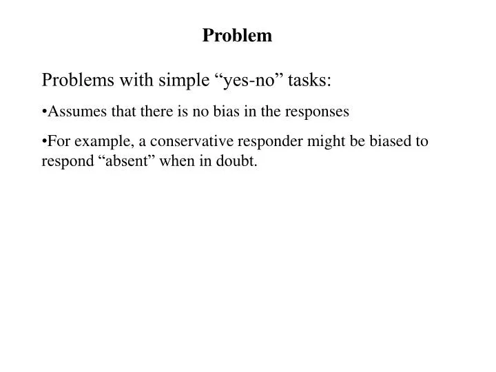
Problem • Problems with simple “yes-no” tasks: • Assumes that there is no bias in the responses • For example, a conservative responder might be biased to respond “absent” when in doubt.
State of the World Noise Signal False Alarm Hit Signal Response Correct Rejection Miss Noise Signal Detection Theory Possible states of the world --signal --noise Possible responses --signal --noise How can we explain a given pattern of responses?
Signal Detection Theory Possible states of the world --signal --noise Possible responses --signal --noise State of the World Medical Terms Noise Signal False Positive Signal True Positive Response True Negative False Negative Noise How can we explain a given pattern of responses?
Signal Detection Theory Possible states of the world --signal --noise Possible responses --signal --noise State of the World Statistical Terms Noise Signal Type-I error () Power (1-) Signal Response Type-II error () . Noise How can we explain a given pattern of responses?
Signal Detection Theory Each trial, stimulus generates an internal (neural) signal.
Signal Detection Theory However, there is also internal noise to deal with.
Signal + Noise Internally, this noise is added to the signal, making the signal noisy… This means that detecting the presence of a signal at low intensities is difficult and error prone.
Signal Detection Theory However, as the signal becomes more intense, the Signal + Noise combination resembles the Noise alone less and less…
Signal Detection Theory However, as the signal becomes more intense, the Signal + Noise combination resembles the Noise alone less and less… …until finally there is very little overlap.
P (X |N) X (Internal Signal) P (X |S) X (Internal Signal) Signal Detection Theory Each trial, stimulus generates an internal (neural) signal, X. Signal and Noise stimuli tend to generate internal signals of different strength
Signal Noise P (X|N or S) X (Internal Signal) Performance is imperfect because signal, noise distributions overlap. How do we decide whether an internal signal X was produced by a signal or by noise?
XC Signal Noise P (X |[N or S+N]) X (Internal Signal) How do we decide whether an internal signal X was produced by a signal or by noise? --Have to establish a criterion, Xc If X < XC, response = Noise If X > XC, response = Signal
XC Noise P (X |[N or S+N]) X (Internal Signal) If a Noise trial produces X > XC, result will be a False Alarm.
XC Signal P (X |[N or S+N]) X (Internal Signal) If a Signal trial produces X < XC, result will be a Miss.
XC P (X |[N or S+N]) Setting XC FAR(False Alarm Rate) = MR(miss rate)
Setting XC XC P (X |[N or S+N]) FAR < MR XC P (X |[N or S+N]) FAR > MR
Setting XC By adjusting XC, we introduce response bias -- Quantified by measure Beta = ratio of signal-to-noise probability that you set as your criterion. -- XC moves left, Beta decreases, responses more liberal -- XC moves right, Beta increases, responses more conservative
Setting XC Bias isn’t (necessarily) bad. -- One state of the world may be more likely than the other -- To minimize errors, responses should favor likely state If the probability that there is a signal increases, then your bias will become smaller. Example: airport x-ray detection -- probability of a weapon is low, so you want to become more conservative and reduce the likelihood that you “cry wolf”
Setting XC -- Responses may have different costs and payoffs -- Goal will be to minimize costs /maximize payoffs V = Value (or payoff/benefit) C = cost
Describes an operator’s performance. Indicate where observer should set criterion. P(X|S) = height of signal curve at proportion corresponding to MR (miss rate) P(X|N) = height of noise curve at proportion corresponding to CRR (correct rejection rate)
Assume…. P(N) = .75 P(S) = .25 V(CR) = V(H) = C(FA) = 1 C(M) = 10 Cost of a miss is high, e.g. terrorist bomb MR = .1 CRR = .8 Then… P(X|S) = .176 P(X|N) = .28 Observed values Observer should be more liberal
P (X) X Mean 1 SD Normal Curve -- mean = median = peak -- spread measured by standard deviation or variance -- a Z-score indicates how many SDs above/below the mean a given value is -- knowing Z-score, we know what proportion of area under the curve is below/above X -- knowing proportion, we can find corresponding Z-score
P (X|N or S) X (Internal Signal) P (X |N or S) X (Internal Signal) Sensitivity -- ease of discriminating N from S -- determined by d’, separation between N and Sdistributions
Calculating d’ -- measured in SDs --if S, N distributions are normal with equal variance, then d’ = Z(Hit Rate) – Z (False Alarm Rate) e.g., if HR = .8 & FAR = .15, the d’ = .84 – (-1.04) = 1.88 -- if distributions are non-normal, or have unequal variances, an alternative measure is necessary (more to come…)
XC P (X |[N or S+N]) XC P (X |[N or S+N]) Sensitivity & Bias In SDT, criterion & sensitivity are independent… …sensitivity reflects perception/encoding (affected by attention) …bias reflects decision making
1.00 HR 0.00 1.00 0.00 FAR By changing bias & keeping d’ constant, we can plot a Receiver Operating Characteristic. Sensitivity is constant along each curve. As d’ increases, ROC curve becomes more bowed.
Z (HR) Z (FAR) ROC curve can also be plotted in Z-scores. d’ is the distance from the chance diagonal to The ROC curve.
ROC curves can be collected... -- by varying payoffs & costs -- by varying probabilities
Why bother with an ROC curve? Tells us whether assumptions for calculating d’ are met. Z (HR) Z (FAR) If assumptions are not met, ROC curve in Z-scores will not be parallel to chance diagonal. When assumptions can not be confirmed, an alternative measure of sensitivity is…
SDT measures of Sensitivity & Bias To measure sensitivity when assumptions are met To measure sensitivity when assumptions can not be confirmed: (area under ROC curve ) To measure bias (May change when d’ changes) (Less sensitive to d’ changes)
Implications of SDT Designing experiments… -- need all four cells of 2 x 2 SDT matrix in order to distinguish effects of sensitivity from effects of bias Understanding real-world phenomena -- change in performance might result from change in sensitivity or change in bias
Implications of SDT Suspect Identification in Police Lineups Stage 1: Is the suspect here? (detection) Stage 2: Which of these people is it? (recognition) If the suspect is actually present, there is no way to estimate the FAR or CRR…and no way to distinguish sensitivity from bias! Experiments show -- witness bias toward “suspect present” response -- witnesses may identify suspect (falsely or correctly) based on characteristics besides memory of crime
Implications of SDT Suspect Identification in Police Lineups Improving performance -- Tell witness that suspect may not be present -- Use a blank lineup control (a noise trial) to weed out witnesses with liberal bias
1.00 HR Z (HR) 0.00 1.00 0.00 FAR Z (FAR)
Information Theory Engineering Psych treats human as information processing system -- Perceive/encode -- Remember -- Communicate How to measure information -- in the environment? -- processed by observer? Information theory provides a system for quantifying information transmitted by a system.
Information Theory Information is reduction of uncertainty following the occurrence of some event. All of the following events convey information -- conclusion of a basketball game -- flashing of the “Door Open” light on car dashboard -- draw of the night’s winning lottery numbers -- pronouncing of the final word in a sentence -- sun rise What determines the amount of information conveyed by an event? -- Number of Possible Events -- Probability of Potential Events -- Context
Information Theory What determines the amount of information conveyed by an event? Number of Possible Events Example: the conclusion of a race will convey more information than the conclusion of a ball game. why? There are more possible winners in a race and only 2 possible in a ball game.
Information Theory What determines the amount of information conveyed by an event? Number of Possible Events -- Information increases as the number of possible events increases. -- If N potential events are equally likely, then the info conveyed by a single event is -- units are bits -- Smallest number of possible events which can produce uncertainty is 2. When N = 2, Hs= 1 -- When N = 1, there is no uncertainty, and Hs= 0
Information Theory Probability of Potential Events -- Information of a single event increases as the likelihood of that event decreases Example: “The July it was hot in Washington” has less information than “The July it snowed in Washington”
Information Theory Probability of Potential Events -- Information of a single event increases as the likelihood of that event decreases -- If the Pi is the probability of event i, then the info conveyed by even i is -- notice that when all events are equally likely, then and
Probability of Events ProbabilityInformation certain 100% = log2(1/1) 0 likely 10% = log2(1/0.1) 3.3 rare 0.1% = log2(1/.001) 9.9 bits
Information Theory Probability of Potential Events -- Average info conveyed by a series of events is -- Note that the average is weighed by the likelihood of the event. -- Therefore, high probability (low information) events will be weighed disproportionately. -- Note that average information is maximal when all events are equally likely
Example: Assume that N = 3 and P1 = .33 P2 = .33 P3 = .33 Total =100% Then HAve = .33 * 1.6 + .33 * 1.6 + .33 * 1.6 = 1.58 Assume that N = 3 and P1 = .8 P2 = .1 P3 = .1 Total =100% Then HAve = .8 * .32 + .1 * 3.32 + .1 * 3.32 = .92
Information Theory Context/Sequential Constraints -- Because some events are more likely under some circumstances than under others, context can modulate information conveyed by an event Example: What is the second letter of each word? T----- Q----- Example: “When I grow up, I want to be a principal or a _____” Low info: policeman, teacher Ralph Wiggum (High info): caterpillar
Information Theory Human can be conceived of as an information channel -- perceives information conveyed by stimulus -- transmits information by making responses If information transmission is perfect, then Transmission may be imperfect because of -- info loss -- noise Channel capacity is the maximum quantity of information that a channel can transmit. HStimulus = HResponse
Information Theory Channel Capacity in Human Performance: Limits on Absolute Judgment -- Absolute judgment task: Each trial, observer identifies or classifies one of several stimuli along a continuum -- Examples include: View one patch of color at a time, and identify it Hear one tone at a time, identify it View lines one at a time, classify length
Information Theory Limits on Absolute Judgment Judgments on One Dimension -- Performance limited to roughly 7 2 items (2 –3 bits of information) for one dimensional judgments Judgments on Multiple Dimensions -- Dimensions may be correlated or orthogonal -- Correlated dimensions convey identical info -- Orthogonal dimensions convey independent info