Download
1 / 76
910 likes | 1.24k Views
The Standard Normal Distribution. PSY440 June 3, 2008. Outline of Class Period. Article Presentation (Kristin M) Recap of two items from last time Using Excel to compute descriptive statistics Using SPSS to generate histograms Standardization (z-transformation) of scores

E N D
The Standard Normal Distribution PSY440 June 3, 2008
Outline of Class Period • Article Presentation (Kristin M) • Recap of two items from last time • Using Excel to compute descriptive statistics • Using SPSS to generate histograms • Standardization (z-transformation) of scores • The normal distribution • Properties of the normal curve • Standard normal distribution & the unit normal table • Intro to probability theory and hypothesis testing
Using Excel to Compute Mean & SD Step 1: Compute mean of height with formula bar. Step 2: Create deviation scores by creating a formula that subtracts the mean from each raw score, and apply the formula to all of the cells in a blank column next to the column of raw scores. Step 3: Square the deviations by creating a formula and applying it to the cells in the next blank column. Step 4: Use the formula bar to add the squared deviations, divide by (n-1) and take the square root of the result. Step 5: Check the result by computing the SD with the formula bar.
Using SPSS to generate histograms Most common answer: Most distinctive answer:
How did this happen? The shape of the histogram will change depending on the intervals used on the x axis. For very large samples and truly continuous variables, the shape will smooth out, but with smaller samples, the shape can change considerably if you change the size of the intervals.
Make sure you are in charge of SPSS and not vice versa! • SPSS has default settings for many of its operations that or may not be what you want. • You can tell SPSS how many intervals you want in your histogram, or how large you want the intervals to be.
Histogram with 16 intervals In legacy dialogues, chose “interactive” and then choose “histogram.” (see note) In chart builder, choose “histogram” then choose “element properties” then click on “set parameters…”
The Z transformation If you know the mean and standard deviation (sample or population – we won’t worry about which one, since your text book doesn’t) of a distribution, you can convert a given score into a Z score or standard score. This score is informative because it tells you where that score falls relative to other scores in the distribution.
Locating a score • Where is our raw score within the distribution? • The natural choice of reference is the mean (since it is usually easy to find). • So we’ll subtract the mean from the score (find the deviation score). • The direction will be given to us by the negative or positive sign on the deviation score • The distance is the value of the deviation score
Reference point Direction m Locating a score X1 - 100= +62 X1 = 162 X2 = 57 X2 - 100= -43
Reference point Below Above m Locating a score X1 - 100= +62 X1 = 162 X2 = 57 X2 - 100= -43
Raw score Population mean Population standard deviation Transforming a score • The distance is the value of the deviation score • However, this distance is measured with the units of measurement of the score. • Convert the score to a standard (neutral) score. In this case a z-score.
X1 - 100= +1.20 50 X2 - 100= -0.86 m 50 Transforming scores • A z-score specifies the precise location of each X value within a distribution. • Direction: The sign of the z-score (+ or -) signifies whether the score is above the mean or below the mean. • Distance: The numerical value of the z-score specifies the distance from the mean by counting the number of standard deviations between X and . X1 = 162 X2 = 57
Transforming a distribution • We can transform all of the scores in a distribution • We can transform any & all observations to z-scores if we know the distribution mean and standard deviation. • We call this transformed distribution a standardized distribution. • Standardized distributions are used to make dissimilar distributions comparable. • e.g., your height and weight • One of the most common standardized distributions is the Z-distribution.
transformation 50 150 m m Xmean = 100 Properties of the z-score distribution = 0
transformation +1 m m X+1std = 150 Properties of the z-score distribution 50 150 = 0 Xmean = 100 = +1
transformation -1 m m X-1std = 50 Properties of the z-score distribution 50 150 +1 = 0 Xmean = 100 = +1 X+1std = 150 = -1
Properties of the z-score distribution • Shape - the shape of the z-score distribution will be exactly the same as the original distribution of raw scores. Every score stays in the exact same position relative to every other score in the distribution. • Mean - when raw scores are transformed into z-scores, the mean will always = 0. • The standard deviation - when any distribution of raw scores is transformed into z-scores the standard deviation will always = 1.
m m transformation 50 150 -1 +1 Z = -0.60 From z to raw score • We can also transform a z-score back into a raw score if we know the mean and standard deviation information of the original distribution. Z = (X - ) --> (Z)( ) = (X - ) --> X = (Z)( ) + X = (-0.60)( 50) + 100 X = 70
Let’s try it with our data To transform data on height into standard scores, use the formula bar in excel to subtract the mean and divide by the standard deviation. Can also choose standardize (x,mean,sd) Show with shoe size Observe how height and shoe size can be more easily compared with standard (z) scores
Z-transformations with SPSS You can also do this in SPSS. Use Analyze …. Descriptive Statistics…. Descriptives …. Check the box that says “save standardized values as variables.”
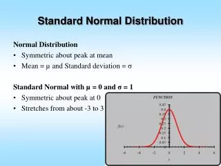
The Normal Distribution • Normal distribution
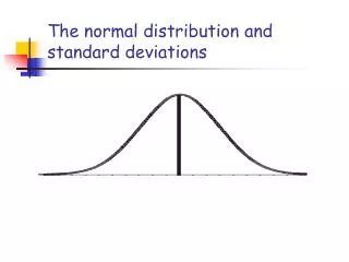
-2 -1 0 1 2 The Normal Distribution • Normal distribution is a commonly found distribution that is symmetrical and unimodal. • Not all unimodal, symmetrical curves are Normal, so be careful with your descriptions • It is defined by the following equation: • The mean, median, and mode are all equal for this distribution.
-2 -1 0 1 2 The Normal Distribution This equation provides x and y coordinates on the graph of the frequency distribution. You can plug a given value of x into the formula to find the corresponding y coordinate. Since the function describes a symmetrical curve, note that the same y (height) is given by two values of x (representing two scores an equal distance above and below the mean) Y =
-2 -1 0 1 2 The Normal Distribution As the distance between the observed score (x) and the mean increases, the value of the expression (i.e., the y coordinate) decreases. Thus the frequency of observed scores that are very high or very low relative to the mean, is low, and as the difference between the observed score and the mean gets very large, the frequency approaches 0. Y =
-2 -1 0 1 2 The Normal Distribution As the distance between the observed score (x) and the mean decreases (i.e., as the observed value approaches the mean), the value of the expression (i.e., the y coordinate) increases. The maximum value of y (i.e., the mode, or the peak in the curve) is reached when the observed score equals the mean – hence mean equals mode. Y =
-2 -1 0 1 2 The Normal Distribution The integral of the function gives the area under the curve (remember this if you took calculus?) The distribution is asymptotic, meaning that there is no closed solution for the integral. It is possible to calculate the proportion of the area under the curve represented by a range of x values (e.g., for x values between -1 and 1). Y =
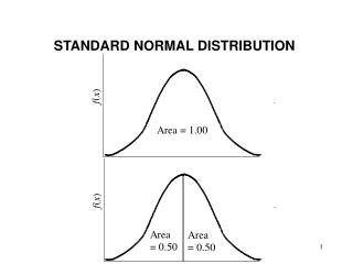
The Unit Normal Table • The normal distribution is often transformed into z-scores. • Gives the precise proportion of scores (in z-scores) between the mean (Z score of 0) and any other Z score in a Normal distribution • Contains the proportions in the tail to the left of corresponding z-scores of a Normal distribution • This means that the table lists only positive Z scores • The .00 column corresponds to column (3) in Table B of your textbook. • Note that for z=0 (i.e., at the mean), the proportion of scores to the left is .5 Hence, mean=median.
34.13% 2.28% 13.59% At z = +1: Using the Unit Normal Table 50%-34%-14% rule Similar to the 68%-95%-99% rule -2 -1 0 1 2 15.87% (13.59% and 2.28%) of the scores are to the right of the score 100%-15.87% = 84.13% to the left
Using the Unit Normal Table • Steps for figuring the percentage above or below a particular raw or Z score: 1. Convert raw score to Z score (if necessary) 2. Draw normal curve, where the Z score falls on it, shade in the area for which you are finding the percentage 3. Make rough estimate of shaded area’s percentage (using 50%-34%-14% rule)
Using the Unit Normal Table • Steps for figuring the percentage above or below a particular raw or Z score: 4.Find exact percentage using unit normal table 5. If needed, subtract percentage from 100%. 6. Check the exact percentage is within the range of the estimate from Step 3
So 90.32% got your score or lower That’s 9.68% above this score SAT Example problems • The population parameters for the SAT are: m = 500, s = 100, and it is Normally distributed Suppose that you got a 630 on the SAT. What percent of the people who take the SAT get your score or lower? • From the table: • z(1.3) =.9032
The Normal Distribution • You can go in the other direction too • Steps for figuring Z scores and raw scores from percentages: 1. Draw normal curve, shade in approximate area for the percentage (using the 50%-34%-14% rule) 2. Make rough estimate of the Z score where the shaded area starts 3. Find the exact Z score using the unit normal table 4. Check that your Z score is similar to the rough estimate from Step 2 5. If you want to find a raw score, change it from the Z score
The Normal Distribution Example: What z score is at the 75th percentile (at or above 75% of the scores)? 1. Draw normal curve, shade in approximate area for the percentage (using the 50%-34%-14% rule) 2. Make rough estimate of the Z score where the shaded area starts (between .5 and 1) 3. Find the exact Z score using the unit normal table (a little less than .7) 4. Check that your Z score is similar to the rough estimate from Step 2 5. If you want to find a raw score, change it from the Z score using mean and standard deviation info.
-2 -1 0 1 2 The Normal Distribution Finding the proportion of scores falling between two observed scores • Convert each score to a z score • Draw a graph of the normal distribution and shade out the area to be identified. • Identify the area below the highest z score using the unit normal table. • Identify the area below the lowest z score using the unit normal table. • Subtract step 4 from step 3. This is the proportion of scores that falls between the two observed scores.
-2 -1 0 1 2 The Normal Distribution Example: What proportion of scores falls between the mean and .2 standard deviations above the mean? • Convert each score to a z score (mean = 0, other score = .2) • Draw a graph of the normal distribution and shade out the area to be identified. • Identify the area below the highest z score using the unit normal table: For z=.2, the proportion to the left = .5793 • Identify the area below the lowest z score using the unit normal table. For z=0, the proportion to the left = .5 • Subtract step 4 from step 3: .5793 - .5 = .0793 About 8% of the observations fall between the mean and .2 SD.
-2 -1 0 1 2 The Normal Distribution Example 2: What proportion of scores falls between -.2 standard deviations and -.6 standard deviations? • Convert each score to a z score (-.2 and -.6) • Draw a graph of the normal distribution and shade out the area to be identified. • Identify the area below the highest z score using the unit normal table: For z=-.2, the proportion to the left = 1 - .5793 = .4207 • Identify the area below the lowest z score using the unit normal table. For z=-.6, the proportion to the left = 1 - .7257 = .2743 • Subtract step 4 from step 3: .4207 - .2743 = .1464 About 15% of the observations fall between -.2 and -.6 SD.
Hypothesis testing • Example: Testing the effectiveness of a new memory treatment for patients with memory problems • Our pharmaceutical company develops a new drug treatment that is designed to help patients with impaired memories. • Before we market the drug we want to see if it works. • The drug is designed to work on all memory patients, but we can’t test them all (the population). • So we decide to use a sample and conduct the following experiment. • Based on the results from the sample we will make conclusions about the population.
Memory treatment Memory Test Memory patients No Memory treatment Memory Test 5 error diff Hypothesis testing • Example: Testing the effectiveness of a new memory treatment for patients with memory problems 55 errors 60 errors • Is the 5 error difference: • A “real” difference due to the effect of the treatment • Or is it just sampling error?
Testing Hypotheses • Hypothesis testing • Procedure for deciding whether the outcome of a study (results for a sample) support a particular theory (which is thought to apply to a population) • Core logic of hypothesis testing • Considers the probability that the result of a study could have come about if the experimental procedure had no effect • If this probability is low, scenario of no effect is rejected and the theory behind the experimental procedure is supported
Basics of Probability • Probability • Expected relative frequency of a particular outcome • Outcome • The result of an experiment
One outcome classified as heads 1 = = 0.5 2 Total of two outcomes Flipping a coin example What are the odds of getting a “heads”? n = 1 flip
One 2 “heads” outcome = 0.25 Four total outcomes Flipping a coin example What are the odds of getting two “heads”? n = 2 Number of heads 2 1 1 0 # of outcomes = 2n This situation is known as the binomial
Three “at least one heads” outcome = 0.75 Four total outcomes Flipping a coin example What are the odds of getting “at least one heads”? n = 2 Number of heads 2 1 1 0
Flipping a coin example Number of heads n = 3 HHH 3 HHT 2 HTH 2 HTT 1 2 THH THT 1 TTH 1 TTT 0 = 23 = 8total outcomes 2n
.4 .3 probability .2 .1 .125 .375 .375 .125 0 1 2 3 Number of heads Flipping a coin example Number of heads Distribution of possible outcomes (n = 3 flips) 3 2 2 1 2 1 1 0
Flipping a coin example Can make predictions about likelihood of outcomes based on this distribution. Distribution of possible outcomes (n = 3 flips) .4 What’s the probability of flipping three heads in a row? .3 probability .2 .1 p = 0.125 .125 .375 .375 .125 0 1 2 3 Number of heads
Flipping a coin example Can make predictions about likelihood of outcomes based on this distribution. Distribution of possible outcomes (n = 3 flips) .4 What’s the probability of flipping at least two heads in three tosses? .3 probability .2 .1 p = 0.375 + 0.125 = 0.50 .125 .375 .375 .125 0 1 2 3 Number of heads
Flipping a coin example Can make predictions about likelihood of outcomes based on this distribution. Distribution of possible outcomes (n = 3 flips) .4 What’s the probability of flipping all heads or all tails in three tosses? .3 probability .2 .1 p = 0.125 + 0.125 = 0.25 .125 .375 .375 .125 0 1 2 3 Number of heads
Hypothesis testing Can make predictions about likelihood of outcomes based on this distribution. Distribution of possible outcomes (of a particular sample size, n) • In hypothesis testing, we compare our observed samples with the distribution of possible samples (transformed into standardized distributions) • This distribution of possible outcomes is often Normally Distributed