Download
1 / 115
1.23k likes | 1.76k Views
The Normal Distribution & Standard Normal Distribution. I The Normal Distribution A What is it? B Why is it everywhere? Probability Theory is why C The Skewed Normal Distribution D Kurtosis II The Standard Normal Distribution A Standardizing a Normal Distribution

E N D
The Normal Distribution & Standard Normal Distribution I The Normal Distribution A What is it? B Why is it everywhere? Probability Theory is why C The Skewed Normal Distribution D Kurtosis II The Standard Normal Distribution A Standardizing a Normal Distribution B Computing Proportions using Table B.1 Anthony J Greene
A Normal Distribution:Chest Sizes of Scottish Militia Men Anthony J Greene
A Normal Distribution:Histogram of Human Gestation Anthony J Greene
The Normal Distribution: Height Anthony J Greene
A Normal Distribution:Age At Retirement Anthony J Greene
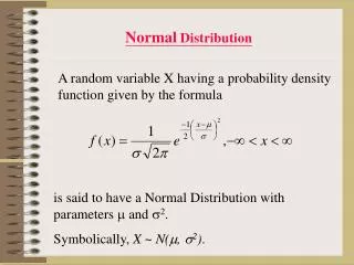
Normally Distributed Variables • The most common continuous (interval/ratio) variable type • Occurs predominantly in nature (biology, psychology, etc.) • Determined by the principles of Probability Anthony J Greene
Probability and the Normal Distribution Probability is the Underlying Cause of the Normal Distribution Anthony J Greene
Possible outcomes for four coin tosses There are 16 possibilities because there are 2 possible outcomes for each toss and 4 tosses: 24 In general the possible outcomes are mn where m is the number of outcomes per event and n is the number of events Anthony J Greene
Probability distribution of the number of heads obtained in 4 coin tosses Anthony J Greene
Probability distribution of the number of heads obtained in 4 coin tosses Anthony J Greene
Frequencies for the numbers of heads obtained in 4 tosses for 1000 observations Anthony J Greene
(a) Probability for 4 coin flips vs. (b) 1000 observations Anthony J Greene
Interpretation of a Normal Distribution in terms of Probability Consider what would happen if there were only 4 genes for height (there are more), each of which has only 2 possible states (like heads versus tails for a coin), call the states T for tall and S for short. The distributions would be identical to that for the coin tosses (see left below) with the possibility of 0, 1, 2, 3, and 4 T’s. In reality height is controlled by many genes so that more than 5 outcomes are possible (see right below).
And for 6 coins instead of 4? Anthony J Greene
Another Example 2 Dice Possible outcomes: 1,1 1,2 1,3 1,4 1,5 1,6 2,1 2,2 2,3 2,4 2,5 2,6 3,1 3,2 3,3 3,4 3,5 3,6 4,1 4,2 4,3 4,4 4,5 4,6 5,1 5,2 5,3 5,4 5,5 5,6 6,1 6,2 6,3 6,4 6,5 6,6 Anthony J Greene
Another Example Anthony J Greene
Age Height Weight I.Q. Sick Days per Year Hours Sleep per Night Words Read per Minute Calories Eaten per Day Hours of Work Done per Day Eyeblinks per Hour Insulting Remarks per Week Number of Pairs of Socks Owned Examples of the Normal Distribution Anthony J Greene
The Skewed Normal Distribution Anthony J Greene
Income Number of Empty Soda Cans in Car Drug Use per Week Car Accidents per Year Lifetime Hospitalizations Number of Guitars Owned Consecutive Days Unemployed Hand-Washings per Day Number of Languages Spoken Fluently Hours of T.V. per Day Examples of Skewed Normal Distributions Anthony J Greene
Graph of a Normal Distribution 34.13% 13.59% 2.28% 34.13% 13.59% 2.28% Anthony J Greene
Shapes of the Normal Distribution Kurtosis • Leptokurtic • Platokurtic Anthony J Greene
Frequency and relative-frequency distributions for heights Anthony J Greene
What do we do with Normal Distributions? • Determine the position of a given score relative to all other scores. • Compare distributions. Anthony J Greene
Relative-frequency histogram for heights Anthony J Greene
Comparing Two Distributions Two distributions of exam scores. For both distributions, µ = 70, but for one distribution, σ = 12. The position of X = 76 is very different for these two distributions. Anthony J Greene
Data Transformations are Reversible and Do not Alter the Relations Among Items 1) Add or Subtract a Constant From Each Score 2) Multiply Each Score By a Constant • e.g., if you wanted to convert a group of Fahrenheit temperatures to Centigrade you would subtract 32 from each score then multiply by 5/9ths Anthony J Greene
Transforming a distribution does not change the shape of the distribution, only its units Anthony J Greene
Height a) in inches b) in centimetersinches X 2.54 = centimeters Anthony J Greene
Transformations Anthony J Greene
Standard Normal Distribution A normally distributed variable having mean 0 and standard deviation 1 is said to have the standard normal distribution. Its associated normal curve is called the standard normal curve. Anthony J Greene
Transformation to Standard Units The idea is to transform (reversibly) any normal distribution into a STANDARD NORMALdistribution with μ = 0 and σ = 1 Anthony J Greene
Standardized Normally Distributed Variable A normally distributed variable, x, is converted to a standard normal distribution, z, with the following formula Anthony J Greene
Standardizing normal distributions Anthony J Greene
Standard Normal Distribution • For a variable x, the variable (z-score) • is called the standardized version of x or the standardized variable corresponding to the variable x. • This transformation is standard for any variable and preserves the exact relationships among the scores Anthony J Greene
Standard Normal Distributions • The z-score transformation is entirely reversible but allows any distribution to be compared (e.g., I.Q. and SAT score; does a top I.Q. score correspond to a top SAT score?) • z-scores all have a mean of zero and a standard deviation of 1, which gives them the simplest possible mathematical properties. Anthony J Greene
Standard Normal Distributions An example of a z transformation from a variable (x) with mean 3 and standard deviation 2 Anthony J Greene
Understanding x and z-scores Anthony J Greene
Basic Properties of the Standard Normal Curve Property 1: The total area under the standard normal curve is equal to 1. Property 2: The standard normal curve extends indefinitely in both directions, approaching, but never touching, the horizontal axis as it does so. Property 3: The standard normal curve is symmetric about 0; that is, the left side of the curve should be a mirror image of the right side of the curve. Property 4: Most of the area under the standard normal curve lies between –3 and 3. Anthony J Greene
Finding percentages for a normally distributed variable from areas under the standard normal curve Because the standard normal distribution is the same for all variables, it is an easy way to determine what proportion of scores is less than a, what proportion lies between a and b, and what proportion is greater than b (for any distribution and any desired points a and b). Anthony J Greene
The relationship between z-score values and locations in a population distribution. Anthony J Greene
The X-axis is relabeled in z-score units. The distance that is equivalent to σ corresponds to 1 point on the z-score scale. Anthony J Greene
Table B.1A Closer Look Anthony J Greene
The Normal Distribution: why use a table? Anthony J Greene
From x or z to PTo determine a percentage orprobability for a normally distributed variable Step 1 Sketch the normal curve associated with the variable Step 2 Shade the region of interest and mark the delimiting x-values Step 3 Compute the z-scores for the delimiting x-values found in Step 2 Step 4 Use Table B.1 to obtain the area under the standard normal curve delimited by the z-scores found in Step 3Use Geometry and remember that the total area under the curve is always 1.00. Anthony J Greene
From x or z to PFinding percentages for a normally distributed variable from areas under the standard normal curve Anthony J Greene
Finding percentages for a normally distributed variable from areas under the standard normal curve • , are given. • a and b are any two values of the variable x. • Compute z-scores for a and b. • Consult table B-1 • Use geometry to find desired area. Anthony J Greene
Given that a quiz has a mean score of 14 and an s.d. of 3, what proportion of the class will score between 9 & 16? • = 14 and = 3. • a = 9 and b = 16. • za = -5/3 = -1.67, zb = 2/3 = 0.67. • In table B.1, we see that the area to the left of a is 0.0475 and that the area to the right of b is 0.2514. • The area between a and b is therefore 1 – (0.0475 + 0.2514) = 0.701 or 70.01% Anthony J Greene
Finding the area under the standard normal curve to the left of z = 1.23 Anthony J Greene
What if you start with x instead of z? What is the probability of selecting a random student who scored above 650 on the SAT? z = 1.50: Use Column C; P = 0.0668 Anthony J Greene