Download
1 / 14
140 likes | 145 Views
CMS Tracker Commissioning. Jennifer Grab Lafayette College, PA, USA Advisors: Drs. Slawomir Tkaczyk and Christophe Delaere. C ompact M uon S olenoid ( CMS ). The Silicon Tracker.

E N D
CMS Tracker Commissioning Jennifer Grab Lafayette College, PA, USA Advisors: Drs. Slawomir Tkaczyk and Christophe Delaere
The Silicon Tracker • Consists of the 3-layer pixel detector and 10 layers of silicon strip detectors assembled in four partitions, TIB, TOB, TEC+, and TEC-. • Total of 220 m2 of silicon crystals 300 and 500 µm thick.
Silicon Strip Detector • The second subsystem after the pixel detector • Contains 15,200 modules with a total of 10 million detector strips read by 80,000 microelectronic chips • Each module consists of strips, a mechanical support structure, and readout electronics. • As a charged particle crosses the material it creates electron-hole pairs that produce a small current lasting a few nanoseconds. • This current is read out and amplified by an Analogue Pipeline Voltage (APV25) chip. Each module has four or six APVs. • Designed to withstand a large amount of radiation
CRAFT 2009 (Cosmic Run At Four Tesla) • Cosmic muon data runs • There are still some noisy modules - more commissioning/calibration required • Opportunity to identify and mask out these modules
Commissioning • Signal-to-noise ratio (SNR or S/N) – the ratio of signal power to noise power • Want to make the SNR as large as possible • If the SNR is not very large, then random fluctuations as a result of noise can obscure the signal • For a long term experiment such as CMS, it is important to have a large SNR since it will decrease over time due to radiation damage effects in the silicon crystals. • Maximize the signal and minimize the noise level • The amount of noise can be determined from pedestal data runs • The noise level is minimized by finding and masking signals from noisy strips in the detector
Noise Analysis – Summary Histograms • Noisy modules can be identified by looking at summary histograms in pedestal runs • 1D Profile histograms – take the mean and standard deviation from each bin in a 2D scatter plot – the bin entry is the mean and the error bars are the standard deviation
Noise Analysis – Summary Histograms • StripNoise histograms plot the mean noise for each module • StripPedestal histograms plot the mean pedestal for each module • Pedestal is the repeated readout from the detector in the absence of a signal • Want to find modules whose noise level is far from the mean and modules with large error
pedestalOutliers.C macro • Analyzes and compares 1D summary histograms from pedestal runs • Want to compare runs from CRAFT 2008 with runs from CRAFT 2009 to see if problems have developed over time • Input – 2 ROOT files taken at different times (CRAFT 2008 and now) • Output – plot overlaying the two histograms, statistics such as standard deviation and mean, a list of outliers (noisy modules) that are in both histograms, and a list of outliers that are in only one of the histograms • Algorithm for finding outliers – • The user can specify whether the macro looks at StripNoise histograms, StripProfile summary histograms, or individual modules • Modules whose noise level is greater than three standard deviations from the mean • A histogram of the error for each bin is created and outliers whose error is more than three standard deviations from the mean are listed
Noise Analysis – Individual Modules • Each module has a set of histograms that cover the strips • Two or three channels per module – each channel has a noise and pedestal profile histogram
moduleComparison.C macro • Input – two ROOT files from CRAFT 2008 and 2009 • Loops over histograms for individual modules and looks for strips that have changed significantly over time • Algorithm for finding strips that have changed • creates a histogram consisting of the ratios of the bin values from the two data runs • Strips with ratios above 1.5 or below 0.5 are listed (strips with a 50% change) • Statistics such as mean and standard deviation are calculated for the ratio histogram and listed for modules with outliers • Outputs a text file listing statistics and outliers for individual modules
What I’ve learned • How to use ROOT to produce and analyze histograms • The C++ programming language • The architecture of and physics behind the CMS tracker • The essentials of noise analysis • Valuable knowledge about particle physics
A special thanks to: • Dr. Slawomir Tkaczyk • Dr. Christophe Delaere • Dr. Jean Krisch • Dr. Homer Neal • Dr. Steven Goldfarb • Dr. Myron Campbell • Jeremy Herr • The University of Michigan • NSF • CERN • Fellow summer students
Are you CERN? This is not Geneva… This is CERN!!! Questions?