Download
1 / 42
450 likes | 986 Views
Measuring Disease Occurrence . Occurrence of disease is the fundamental outcome measurement of epidemiology Occurrence of disease is typically a binary (yes/no) outcome Occurrence of disease involves time. Main Points to be Covered. Incidence versus Prevalence

E N D
Measuring Disease Occurrence • Occurrence of disease is the fundamental outcome measurement of epidemiology • Occurrence of disease is typically a binary (yes/no) outcome • Occurrence of disease involves time
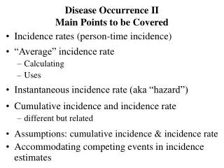
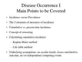
Main Points to be Covered • Incidence versus Prevalence • The 3 elements of measures of incidence • Cumulative vs. person-time incidence • Calculating cumulative incidence by the Kaplan-Meier method • Calculating cumulative incidence by the life table method
Prevalence versus Incidence • Prevalence counts existing disease diagnoses, usually at a single point in time • Incidence counts new disease diagnoses during a defined time period
Two Types of Prevalence • Point prevalence - number of persons with a specific disease at one point in time divided by total number of persons in the population • Period prevalence - number of persons with disease in a time interval (eg, one year) divided by number of persons in the population • Prevalence at beginning of an interval plus any incident cases • Risk factor prevalence may also be important
Example of Point Prevalence • NHANES = National Health and Nutrition Examination Survey, a probability sample of all U.S. residents from 1988 to 1994 • During NHANES III, blood samples drawn and tested for antibodies against HIV • Estimated national prevalence: 461,000 HIV-infected (0.18%) McQuillan et al., JAIDS, 1997
Example of Period Prevalence: National Health Interview Survey (NHIS)
The Three Elements in Measures of Disease Incidence • E = an event = a binary outcome • N = number of at-risk persons in the population under study • T = time period during which the events are observed
Disease Occurrence Measures: A Confusion of Terms • Terminology is not standardized and is used carelessly even by those who know better • Key to understanding measures is to pay attention to how the 3 elements of number of events (E), number of persons at risk (N), and time (T) are used • Even the basic difference between prevalence and incidence is often ignored
Incidence or Prevalence? HIV/AIDS infection rates drop in Uganda KAMPALA, Sept. 10 (Kyodo) - Infection rates of the HIV/AIDS epidemic among Ugandan men, women and children dropped to 6.1% at the end of 2000 from 6.8% a year earlier, an official report shows. The report, compiled by the Ministry of Health together with the World Health Organization and the Medical Research Council of Britain, says the results were obtained after testing the blood of women attending clinics in 15 hospitals around the country. The ministry deduced the figures for men and children from the blood tests on women, according to the report. The report says the average rate of infection for urban areas fell from 10.9% to 8.7%. In rural areas, the average was 4.2%, not much different from the 4.3% average a year earlier. The highest infection rate of 30% was last reported in western Uganda in 1992.
The word “rate” should be avoided when existing diagnoses at one point in time are what was measured. Although you may encounter “prevalence rate,” rate should be reserved for measuring incidence. In general a rate is a change in one measure with respect to change in a 2nd
Measures that are sometimes loosely called Incidence • Count of the number of events (E) • eg, there were 84 traffic fatalities during the holidays • Count of the number of events during some time period (E/T) • eg, traffic accidents have averaged 50 per week during the past year • Neither explicitly includes the number of persons (N) giving rise to the events
CDC: Chickenpox rates drop in four states as inoculations become common SF Chronicle, Thursday, September 18, 2003 (09-18) 13:51 PDT ATLANTA (AP) -- The number of chickenpox cases in four states dropped more than 75 percent as inoculations became more common in the last decade, according to a federal study released Thursday. The total number of casesin Illinois, Michigan, Texas and West Virginiadropped from about 102,200 in 1990 to about 24,500 in 2001, the Centers for Disease Control and Prevention said. At the same time, the percentage of infants receiving chickenpox shots rose from less than 9 percent in 1996 to as much as 83 percent in 2001, the CDC said.
Problem: How would you measure the occurrence of new cases of breast cancer in a cohort study (such as the Nurses Health Study)?Occurrence of new cases = breast cancer incidence
Two Measures Described as Incidence in the Text • The proportion of individuals who experience the event in a defined time period (E/N during some time T) = cumulative incidence • The number of events divided by the amount of person-time observed (E/NT) = incidencerate or density (not a proportion)
E/N E/T E/NT E
Disease Incidence Key Concept • Numerator is always the number of new events in a time period (E) • Examine the denominator (persons or person-time) to determine the type of incidence measure
Cumulative Incidence • Perhaps most intuitive measure of incidence since it is just proportion of those observed who got the disease • Proportion=probability=risk • Basis for Survival Analysis • Two primary methods for calculating • Kaplan-Meier method • Life table method
Calculating Cumulative Incidence • With complete follow-up cumulative incidence is just number of events (E) divided by the number of persons (N) = E/N • Outbreak investigations, such as of gastrointestinal illness, typically calculate “attack rates” with complete follow-up on a “cohort” of persons who were exposed at the beginning of the epidemic.
Example of using denominator with complete follow-up On June 24, 1996, the Livingston County (New York) Department of Health (LCDOH) was notified of a cluster of diarrheal illness following a party on June 22, at which approximately 30 persons had become ill …. Plesiomonas shigelloides and Salmonella serotype Hartford as the cause of the outbreak… 98 attendees (52%) were interviewed. Sixty persons reported illness. 56 (57%) of 98 respondents had illnesses meeting the case definition. MMWR, May 22, 1998
Cumulative incidence with differing follow-up times • Calculating cumulative incidence in a cohort • Subjects have different starting dates • Subjects have different follow-up after enrollment • Most cohorts have a single ending date but different starting dates for participants because of the recruitment process • Guarantees there will be unequal follow-up time • In addition, very rare not to have drop outs
Calculating Cumulative Incidence with differing follow-up times • The Problem: Since rarely have equal follow-up on everyone, can’t just divide number of events by the number who were initially at risk • The Solution: Kaplan-Meier and life tables are two methods devised to calculate cumulative incidence among persons with differing amounts of follow-up time
Cumulative incidence with Kaplan-Meier estimate • Requires date last observed or date outcome occurred on each individual (end of study can be the last date observed) • Analysis is performed by dividing the follow-up time into discrete pieces • calculate probability of survival at each event (survival = probability of no event)
3 Ways Censoring Occurs 1) Death (if death is not the study outcome) 2) Loss to follow-up (refuse, move, can’t be found) 3) End of study observation (if still alive and haven’t experienced outcome) • Each subject either experiences the outcome or is censored
c Assumption: No temporal/secular trends affecting incidence
Cumulative Incidence Key Concept #1 • To calculate a valid cumulative incidence with different follow-up times, there is the implicit assumption that the probability of the outcome event is not changing during the study period; i.e., there are no temporal/secular trends affecting the outcome.
Calculating Cumulative Incidence • Probability of two independent events occurring is the product of the two probabilities for each occurring alone • eg, if event 1 occurs with probability 1/6 and event 2 with probability 1/2, then the probability of both event 1 and 2 occurring = 1/6 x 1/2 = 1/12 • Probability of living to time 2 given that one has already lived to time 1 is independent of the probability of living to time 1
Cumulative survival calculated by multiplying probabilities for each prior failure time: e.g., 0.9 x 0.875 x 0.857 = 0.675 and 0.9 x 0.875 x 0.857 x 0.800 x 0.667 x 0.500 = 0.180
Kaplan-Meier Cumulative Incidence of the Outcome • Cannot calculate by multiplying each event probability (=probability of repeating event) • (in our example, 0.100 x 0.125 x 0.143 x 0.200 x 0.333 x 0.500 = 0.0000595) • Obtain by subtracting cumulative probability of surviving from 1; eg, (1 - 0.180) = 0.82 • Since it is a proportion, it has no time unit connected to it, so time period has to be added; e.g, 2-year cumulative incidence
Survival After Breast Cancer in Ashkenazi Jewish BRCA1 and BRCA2 Mutation Carriers Lee et al., JNCI 1999
Kaplan-Meier using STATA Need a data set with one observation per person. Each person either experiences event or is censored. Need a variable for the time from study entry to date of event or date of censoring/failure (timevariable). Need a variable indicating whether follow-up ended with the event or with censoring/failure (failvariable)
All of preceding can be done in STATA 9 using its pull-down menus. Statistics Survival Analysis Setup & Utilities Use Declare data to be survival-time data to identify time and censoring variables and specify value that indicates failure (eg, 1) Statistics Survival Analysis Summary statistics, tests, & tables Use Create survivor, hazard, & other variables to get values of survival function Use Graph survivor & cumulative hazard functions to get K-M graph (or use pull-down Graphics--Survival analysis graphs)
Cumulative Incidence Key Concept #2 • Censoring is unrelated to the probability of experiencing the outcome (unrelated to survival)
Preservation of glomerular filtration rate on dialysis when adjusted for patient dropout. BACKGROUND: Residual renal function (RRF) plays an important role in dialysis patients. … We speculated that regardless of the patient's type of therapy, the estimate obtained for the rate of decline in glomerular filtration rate (GFR) may be biased because of informative censoring associated with patient dropout. Informative censoring occurs when patients who die or transfer to another modality very early have associated with them a lower starting GFR or a higher rate of decline of GFR than patients who either complete the study or who die or transfer much later. If patient dropout is indeed related to the rate of decline in GFR and if this relationship is ignored in the analysis, then the estimate obtained of the rate of decline in GFR may be biased. …The results show that for the CANUSA cohort, the mean initial GFR was significantly lower, and the rate of decline was significantly higher for patients who died or transferred to HD than for patients who were randomly censored or received a transplant. CONCLUSION: In any longitudinal study designed to estimate trends in an outcome measured over time, it is important that the analysis of the data takes into account any effect patient dropout may have on the estimated trend. This analysis demonstrates that among PD patients, both the starting GFR and the rate of decline in GFR are associated with patient dropout. Misra et al., Kidney Int 2000
Life table method of estimating cumulative incidence • Key difference from Kaplan-Meier is that probabilities are calculated for fixed time intervals, not at the exact time of each event • Unlike Kaplan-Meier, don’t need to know date of each event • For large data sets the life table and the Kaplan-Meier method produce nearly the same results
Life table method • Fixed time intervals can vary in length but are often uniform • Probability of surviving each fixed time interval is calculated • Cumulative survival is product of probabilities from each prior time period
Life table method of estimating cumulative incidence • Since exact event times not used, assumption that events and censoring occur uniformly during the fixed time intervals • Calculations are based on assigning censored individuals follow-up for half of the time period (follows from uniformity assumption) • Subtract one-half of subjects lost during interval from denominator at interval beginning
Summary Points • Prevalence counts existing disease and incidence counts new diagnoses of disease • Word “rate” is often used incorrectly • Two main types of incidence • incidence based on proportion of persons = cumulative incidence • incidence based on person-time = incidence rate • Kaplan-Meier or life table estimates cumulative incidence assuming losses unrelated to outcome and no temporal trends in outcome incidence