Download
1 / 67
700 likes | 968 Views
Disease Occurrence I Main Points to be Covered. Incidence versus Prevalence The 3 elements of measures of incidence Cumulative vs. person-time incidence Concept of censoring Calculating cumulative incidence Kaplan-Meier method Life table method

E N D
Disease Occurrence IMain Points to be Covered • Incidence versus Prevalence • The 3 elements of measures of incidence • Cumulative vs. person-time incidence • Concept of censoring • Calculating cumulative incidence • Kaplan-Meier method • Life table method • Underlying assumptions: no secular trends, losses unrelated to outcome, no (or independent) competing events
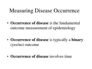
Measuring Disease Occurrence • Occurrence of disease is the fundamental outcome measurement of epidemiology • Occurrence of disease is typically a binary (yes/no) outcome • Note: Continuous changes related to disease, e.g., changes in blood pressure, are also relevant but not the focus of this course • Occurrence of disease involves time
Prevalence versus Incidence • Prevalence counts existing disease diagnoses, usually at a single point in time • Incidence counts new disease diagnoses during a defined time period • Fundamental distinction in epidemiology
Prevalence vs Incidence • Prevalence • Burden of disease -> public health planning • Incidence • Trends over time -> public health implications • Fundamental for studies of causality • Exclude prevalent cases to focus on causes of disease, separate from causes of “survival with disease”
Two Types of Prevalence • Point prevalence - number of persons with a specific disease at one point in time divided by total number of persons in the population • Period prevalence - number of persons with disease in a time interval (eg, one year) divided by number of persons in the population • Prevalence at beginning of an interval plus any incident cases • Risk factor (exposure) prevalence may also be important
Example of Point Prevalence • NHANES = National Health and Nutrition Examination Survey, a probability sample of all U.S. residents, conducted 1988 to 1994 • During NHANES, blood samples drawn and tested for antibodies against HIV • Prevalence of HIV infection = 0.18% McQuillan et al., JAIDS, 1997
Concussion and Cognitive Impairment in Retired Football Players FIGURE 3. Percentage of retired players aged 50 years or older with a diagnosis of MCI and memory problems (self-reported and reported by a spouse or close relative) by concussion history (none, one, two, and three or more). Error bars indicate 95% confidence intervals. P 0.007. Guskiewicz et al.Neurosurgery 2005
Example of Period Prevalence: National Health Interview Survey (NHIS)
How to report prevalence • Prevalence should always be stated as a number between 0 and 1 (e.g., 0.03) or as a percentage (e.g., 3%) • Avoid statements such as: “Prevalence was 0.13 per 1000 persons” Easily confused with a report of incidence Prefer: “Prevalence was 0.013% or 0.00013”
The Three Elements in Measures of Disease Incidence • E = an event = a binary outcome (occurrence of disease) • N = number of at-risk persons in the population under study • T = time period during which the events are observed
Disease Occurrence Measures: A Confusion of Terms • Terminology is not standardized and is used carelessly even by those who know better • Key to understanding measures is to pay attention to how the 3 elements of number of events (E), number of persons at risk (N), and time (T) are used • Even the basic difference between prevalence and incidence is often ignored
Incidence or Prevalence? HIV/AIDS infection rates drop in Uganda KAMPALA, Sept. 10 (Kyodo) - Infection rates of the HIV/AIDS epidemic among Ugandan men, women and children dropped to 6.1% at the end of 2000 from 6.8% a year earlier, an official report shows… The report says the average rate of infection for urban areas fell from 10.9% to 8.7%. In rural areas, the average was 4.2%, not much different from the 4.3% average a year earlier.
“Rate” should be avoided when describing prevalence. • Although you may encounter “prevalence rate,” including in our text, rate should be reserved for measuring incidence. • In general, a rate is a change in one measure with respect to change in a 2nd
Measures that are sometimes loosely called incidence • Count of the number of events (E) • eg, there were 84 traffic fatalities during the holidays • Count of the number of events during some time period (E/T) • eg, traffic accidents have averaged 50 per week during the past year • Neither explicitly includes the number of persons (N) giving rise to the events
CDC: Chickenpox rates drop in four states as inoculations become commonSF Chronicle, Thursday, September 18, 2003 The number of chickenpox cases in four states dropped more than 75 percent as inoculations became more common in the last decade, according to a federal study released Thursday. The total number of cases in Illinois, Michigan, Texas and West Virginia dropped from about 102,200 in 1990 to about 24,500 in 2001, the Centers for Disease Control and Prevention said. At the same time, the percentage of infants receiving chickenpox shots rose from less than 9 percent in 1996 to as much as 83 percent in 2001, the CDC said.
Problem: How would you measure breast cancer incidence in a cohort study (such as the Nurses Health Study)?Disease incidence is the occurrence of new cases over time.But how to account for the role of time?
Cohort study design D = disease occurrence; arrow = losses to follow-up
Two Measures of Incidence • The proportion of individuals who experience the event in a defined time period (E/N during some time T) = cumulative incidence = incidence proportion • The number of events divided by the amount of person-time observed (E/NT) = incidencerate or density (not a proportion)
Cumulative Incidence • Definition: The proportion of individuals who experience the event in a defined time period (E/N during some time T) = cumulative incidence • Example: Diabetic Medications and Fracture: “The cumulative incidence of a first fracture among women reached 15.1% at 5 years with rosiglitazone, 7.3% with metformin, and 7.7% with glyburide.”
Incidence Rate • Definition: The number of events divided by the amount of person-time observed (E/NT) = incidencerate or density (not a proportion) • Same example, Diabetic Medications and Fracture, now presented as incidence rates: “The incidence of a first fracture among women was 2.74 per 100 person-years with rosiglitazone, 1.54 per 100 person-years with metformin, and 1.29 per 100 person-years with glyburide.”
Counterintuitive Idea #2 • The denominator for incidence does not have to be a count of individual persons
E/NT E/N E E/T
Disease Incidence Key Concept • Numerator is always the number of new events in a time period (E) • Examine the denominator (persons or person-time) to determine the type of incidence measure
Cumulative Incidence • Perhaps most intuitive measure of incidence since it is just proportion of those observed who got the disease • Proportion=probability=risk • Over a specific time period
Calculating Cumulative Incidence • With complete and equal follow-up, cumulative incidence is just number of events (E) divided by the number of persons (N) = E/N • Outbreak investigations, such as of gastrointestinal illness, typically calculate “attack rates” (misnomer) with complete follow-up on a “cohort” of persons who were exposed at the beginning of the epidemic.
Denominator with complete and equal follow-up On June 24, 1996, the Livingston County (New York) Department of Health (LCDOH) was notified of a cluster of diarrheal illness following a party on June 22…. Plesiomonas shigelloides and Salmonella serotype Hartford were identified as the cause of the outbreak… 98 attendees were interviewed. 56 (57%) of 98 respondents had illnesses meeting the case definition. MMWR, May 22, 1998
Cumulative incidence with differing follow-up times • Calculating cumulative incidence in a cohort • Subjects have different starting dates • Subjects have different follow-up after enrollment • Most cohorts have a single ending date but different starting dates for participants because of the recruitment process • Guarantees there will be unequal follow-up time • Very rare not to have drop outs, including in trials
Calculating cumulative incidence with differing follow-up times • The Problem: Since rarely have equal follow-up on everyone, can’t just divide number of events by the number who were initially at risk • The Solution: Kaplan-Meier and life tables are two methods devised to calculate cumulative incidence among persons with differing amounts of follow-up time
Cumulative Incidence, not Proportion with Outcome • Previous example: “The cumulative incidence of a first fracture reached 15.1% at 5 years with rosiglitazone, 7.3% with metformin, and 7.7% with glyburide.” Takes into account different follow-up times. We’ll see how to do this in the next slides. • “Among the 1,840 women, 111 reported a first fracture: 60 (9.3%) of those treated with rosiglitazone, 30 (5.1%) of those treated with metformin, and 21 (3.5%) of those treated with glyburide.” The numbers of cases reported in this sentence is useful but the proportions are not. Does not take into account different follow-up times.
Cumulative incidence with Kaplan-Meier estimate • Also called “product limit estimator.” Original article is in the optional reading. • Requires date last observed or date outcome occurred on each individual (end of study can be the last date observed) • Analysis is performed by dividing the follow-up time into discrete pieces • calculate probability of survival at each event (survival = probability of no event)
Two Ways Censoring Occurs 1) Loss to follow-up (refuse, move, can’t be found) 2) End of study (alive and hasn’t experienced outcome) = Administrative Censoring • With all-cause mortality as the outcome, each subject either experiences the outcome or is censored. No competing events.
Calculating Cumulative Incidence • Probability of 2 independent events occurring is the product of the probabilities for each occurring alone • If event 1 occurs with probability 1/6 and event 2 with probability 1/2, then the probability of both event 1 and 2 occurring = 1/6 x 1/2 = 1/12 • Probability of living to time 2 given that one has already lived to time 1 (i.e. conditional on survival to time 1) is independent of the probability of living to time 1
Cumulative survival calculated by multiplying probabilities for each prior failure time: e.g., 0.9 x 0.875 x 0.857 = 0.675 and 0.9 x 0.875 x 0.857 x 0.800 x 0.667 x 0.500 = 0.180
Kaplan-Meier Cumulative Incidence of the Outcome • Cannot calculate by multiplying each event probability (=probability of repeating event) • (in our example, 0.100 x 0.125 x 0.143 x 0.200 x 0.333 x 0.500 = 0.0000595) • Subtract cumulative probability of surviving from 1; e.g., (1 - 0.180) = 0.82 • Proportion, so time is not intrinsic to the units. Time period has to be added for number to be interpretable. e.g., 2 year cumulative incidence.
Examples of Kaplan-Meier Plots Used in observational studies and clinical trials Can be presented as cumulative incidence or cumulative survival
“The cumulative incidence of a first fracture reached 15.1% at 5 years with rosiglitazone, 7.3% with metformin, and 7.7% with glyburide.”
Cumulative incidence of primary CHD events in the HERS trial Log rank P value = 0.91 The number of women observed at each year of follow-up and still free of an event are provided in parentheses, and the curves become fainter when this number drops below half of the cohort. Hulley et al JAMA 1998
Cumulative survival after diagnosis of HIV infection in three groups of patients Tillmann, NEJM 2001
Time Element in Cumulative Incidence • KM plot provides time element - full disclosure on incidence. • However, if you cannot show a plot and you must say cumulative incidence in words, then YOU MUST ADD a TIME ELEMENT. • 5% cumulative incidence of cancer recurrence over 1 year, or over 5 years.
Cumulative Incidence: Underlying Assumption #1 • To calculate cumulative incidence with different follow-up times, we “shifted everyone to the left” and used follow-up time rather than calendar time. • This assumes the probability of the outcome is not changing over calendar time. • i.e. No temporal/secular trends affecting the outcome. • If this assumption is not correct, you can still do the calculation, but the result no longer has a meaningful interpretation.
Underlying secular trends • True changes in incidence • Rapid changes in HIV incidence at start of epidemic • Changes in incidence of hip fracture • Changes in diagnosis or screening • Adding A1C to diagnostic criteria for diabetes • Widespread use of mammography for breast cancer screening • More important in a study with longer follow-up time
FIG. 1. Observed cumulative incidence of any fracture among 1,964 Rochester, MN, residents after first recognition of diabetes mellitus in 1970–1994 Melton et al. JBMR 2008.
Hip fracture trends in Sweden Rogmark et al. Acta Orthop Scand 1999
Cumulative Incidence: Underlying Assumption #2 • For cumulative incidence to be unbiased (i.e. valid), censoring must be unrelated to the probability of experiencing the outcome. • i.e., The experience of those who are lost to follow-up must be the same as those who remain in the study.
Informative vs Non-informative Censoring • Informative censoring (aka Non-ignorable) means that losses to follow-up have different incidence of the outcome than subjects who remain in the study, and therefore introduce bias in the incidence measure • Non-informative censoring (aka Ignorable) means that losses to follow-up have the same incidence of the outcome as subjects who remain in the study, and therefore do not result in bias