Download
1 / 13
130 likes | 276 Views
Angular Velocity: Sect. 1.15 Overview only. For details, see text!. Consider a particle moving on arbitrary path in space: At a given instant, it can be considered as moving in a plane, circular path about an axis Instantaneous Rotation Axis .

E N D
Angular Velocity: Sect. 1.15Overview only. For details, see text! • Consider a particlemoving on arbitrary path in space: • At a given instant, it can be considered as moving in a plane, circular path about an axis Instantaneous Rotation Axis. In an infinitesimal time dt, the path can be represented as infinitesimal circular arc. • As the particle moves in circular path, it has angular velocity: ω (dθ/dt) θ
Consider a particle moving in an instantaneously circular path of radius R. (See Fig.): • Magnitude of Particle Angular Velocity: ω (dθ/dt) θ • Magnitude of Linear Velocity (linear speed): v = R(dθ/dt) = Rθ = Rω
Particle moving in circular path, radius R. (Fig.): Angular Velocity: ωθ Linear Speed:v = Rω (1) • Vector direction of ω normal to the plane of motion, in the direction of a right hand screw. (Fig.). Clearly: R = r sin(α) (2) (1) & (2) v = rωsin(α) So (for detailed proof, see text!): v =ω r
Gradient (Del) Operator:Sect. 1.16Overview only. For details, see text! • The most important vector differential operator: grad • A Vector which has components which are differential operators. Gradient operator. • In Cartesian (rectangular) coordinates: ∑i ei (∂/∂xi) (1) • NOTE!(For future use!) is much more complicated in cylindrical & spherical coordinates (see Appendix F)!!
can operate directly on a scalar function ( gradient of Old Notation: = grad): = ∑i ei (∂/∂xi) A VECTOR! • can operate in a scalar product with a vectorA ( divergence of A; Old: A = div A): A = ∑i (∂Ai/∂xi) A SCALAR! • can operate in a vector product with a vectorA ( curl of A; Old: A = curl A): (A)i = ∑j,k εijk(∂Ak/∂xj) A VECTOR! (Older: A = rot A)Obviously, A = A(x,y,z)
Physical interpretation of the gradient : (Fig) • The text shows that has the properties: 1. It is surfaces of constant 2. It is in the direction of max change in 3. The directional derivative of for any direction n is n = (∂/∂n) (x,y) Contour plot of (x,y)
The Laplacian Operator • The Laplacian is the dot product of with itself: 2 ; 2 ∑i (∂2/∂xi2) A SCALAR! • The Laplacian of a scalar function 2 ∑i (∂2/∂xi2)
Integration of Vectors: Sect. 1.17Overview only. For details, see text! • Types of integrals of vector functions: A = A(x,y,z) = A(x1,x2,x3) = (A1,A2,A3) • Volume Integral(volume V, differential volume element dv) (Fig.): ∫V A dv (∫V A1dv, ∫V A2dv, ∫V A3dv)
Surface Integral(surface S, differential surface element da) (Fig.) ∫S An da, n Normal to surface S
Line integral(path in space, differential path element ds) (Fig.): ∫BC Ads ∫BC∑i Ai dxi
Gauss’s Theorem or Divergence Theorem(for a closed surface S surrounding a volume V) See figure; n Normal to surface S ∫S An da = ∫VA dv Physical Interpretationof A The net “amount” of A “flowing” in & out of closed surface S
Stoke’s Theorem(for a closed loop C surrounding a surface S) See Figure; n Normal to surface S ∫C Ads = ∫S (A)n da Physical Interpretationof A The net “amount” of “rotation” of A