Download
1 / 28
370 likes | 755 Views
Vorticity. In physical oceanography, we deal mostly with the vertical component of vorticity, which is notated as. For a rotating solid object, the vorticity is two times of its angular velocity. Relative vorticity is vorticity relative to rotating earth

E N D
Vorticity In physical oceanography, we deal mostly with the vertical component of vorticity, which is notated as For a rotating solid object, the vorticity is two times of its angular velocity Relative vorticity is vorticity relative to rotating earth Absolute vorticity is the vorticity relative to an inertia frame of reference (e.g., the sun) Planetary vorticity is the part of absolute vorticty associated with Earth rotation f=2sin, which is only dependent on latitude. Absolute vorticity =Relative vorticity + Planetary Vorticity
Vorticity Equation From horizontal momentum equation, , (1) (2) Taking , we have
Shallow Water Equation Constant and uniform density , incompressible Aspect ratio hydrostatic
Integrating the hydrostatic equation Use the boundary condition at the sea surface, z=, p=0 The horizontal pressure gradient is independent of z Therefore, it is consistent to assume that the horizontal velocities remain to be independent of z if they are so initially.
Assume that at the bottom of the sea, i.e., z=-hB At the sea surface, z=,
Let be the total depth of water, we have The system of the shallow water equations
Vorticity Equation for the Shallow Water System >> x, y
Potential Vorticity Conservation For a layer of thickness H, consider a material column We get or Potential Vorticity Equation
Alternative derivation of Sverdrup Relation Construct vorticity equation from geostrophic balance (1) Assume =constant (2) Integrating over the whole ocean depth, we have
where is the entrainment rate from the surface Ekman layer at 45oN The Sverdrup transport is the total of geostrophic and Ekman transport. The indirectly driven Vg may be much larger than VE.
In the ocean’s interior, for large-scale movement, we have the differential form of the Sverdrup relation i.e., <<f
Assume geostrophic balance on -plane approximation, i.e., ( is a constant) Vertically integrating the vorticity equation barotropic we have The entrainment from bottom boundary layer The entrainment from surface boundary layer We have where
Quasi-Geostrophic Approximation Replace the relative vorticity by its geostrophic value Approximate the horizontal velocity by geostrophic current in the advection terms Under -plane approximation, f=fo+y, we have
Quasi-geostrophic vorticity equation and , we have For and where (Ekman transport is negligible) Moreover, We have where
Boundary Value Problem Boundary conditions on a solid boundary L (1) No penetration through the wall (2) No slip at the wall
Non-dimensional vorticity equation Non-dimensionalize all the dependent and independent variables in the quasi-geostrophic equation as where For example, The non-dmensional equation where , nonlinearity. , , , bottom friction. , lateral friction. ,
Interior (Sverdrup) solution If <<1, S<<1, and M<<1, we have the interior (Sverdrup) equation: (satistfying eastern boundary condition) (satistfying western boundary condition) Example: Let , . Over a rectangular basin (x=0,1; y=0,1)
Westward Intensification It is apparent that the Sverdrup balance can not satisfy the mass conservation and vorticity balance for a closed basin. Therefore, it is expected that there exists a “boundary layer” where other terms in the quasi-geostrophic vorticity is important. This layer is located near the western boundary of the basin. Within the western boundary layer (WBL), , for mass balance The non-dimensionalized distance is , the length of the layer <<L In dimensional terms, The Sverdrup relation is broken down.
The Stommel model Bottom Ekman friction becomes important in WBL. , S<<1. at x=0, 1; y=0, 1. No-normal flow boundary condition (Since the horizontal friction is neglected, the no-slip condition can not be enforced. No-normal flow condition is used). Interior solution
Re-scaling in the boundary layer: , we have Let Take into As =0, =0. As ,I
The solution for is , . A=-B , ( can be the interior solution under different winds) For , , . For , , .
The dynamical balance in the Stommel model In the interior, Vorticity input by wind stress curl is balanced by a change in the planetary vorticity f of a fluid column.(In the northern hemisphere, clockwise wind stress curl induces equatorward flow). In WBL, , Since v>0 and is maximum at the western boundary, the bottom friction damps out the clockwise vorticity. Question: Does this mechanism work in a eastern boundary layer?
If f is not constant, then F is dissipation of vorticity due to friction