Download
1 / 17
190 likes | 567 Views
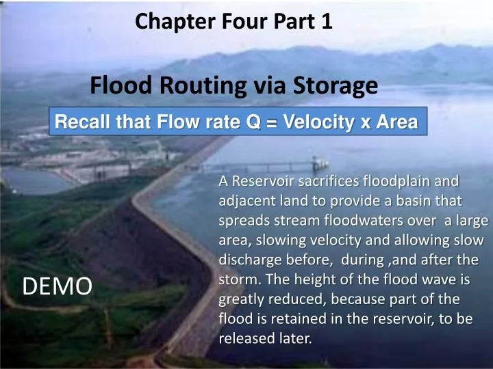
Recall that Flow rate Q = Velocity x Area. Chapter Four Part 1 Flood Routing via Storage.

E N D
Recall that Flow rate Q = Velocity x Area Chapter Four Part 1Flood Routing via Storage A Reservoir sacrifices floodplain and adjacent land to provide a basin that spreads stream floodwaters over a large area, slowing velocity and allowing slow discharge before, during ,and after the storm. The height of the flood wave is greatly reduced, because part of the flood is retained in the reservoir, to be released later. DEMO
Lag due to travel time and filling of reservoir Inflow and outflow hydrographs plotted on same graph. Area A volume of water that fills reservoir, dS/dt > 0. Due to inflow, which is due to precip. At t1 reservoir is full and inflow = outflow.Area C is the volume of water that flows out. If inflow has slowed (storm is past) outflow can be slow. dS/dt < 0, so water in reservoir drops. Outflow rate mostly depends on reservoir water depth, sqrt (2gh), but the spillway operator can lessen it. Units of Storage acre x feet
Most reservoirs have spillways to slowly lower levels in prep for next storm; slow enough not to flood the downstream valley.
Example 4.1 in part DS/Dt = Inflow – Outflow Storage change is equal to the area between the inflow and outflow hydrographs.
Example 4.1 in part • Time (days) I (cfs) Q(cfs) DS/Dt (cfs) • 0.5 500 250 250 • 1.5 3500 1000 2500 • 2.5 9000 3000 6000 • 3.5 9750 4500 5250 • 4.5 8000 5750 2250 • 5.5 4500 6000 -1500 • 6.5 2250 5250 -3000 • 7.5 1250 4250 -3000 • 8.5 250 3250 -3000 • 9.5 0 2500 -2500 • 10.5 0 1500 -1500 • 11.5 0 1000 -1000 • 12.5 0 750 -750 • 13.5 0 0 0 Inflow peaks at 3.5 days, Outflow peaks at 5.5 days, much later and at a much smaller flow rate. At about 5 days, Storage change is zero and storage volume is maximum.
River Routing • Rivers store water on their floodplains. Because the area is so large compared to the channel, floodplain velocities are much slower than channel flows, Q = VA. • Building on floodplains defeats their natural purpose as flood control devices, and ultimately requires expensive flood control projects to prevent flood losses. House Corps of Engineers Project with your tax dollars
River Routing • For natural rivers the attenuation process is more complex than for reservoirs with dams. Take, for example, the 1993 Upper Mississippi floods. We know that great portions of the Upper Mississippi valley were flooded, yet by the time the flood arrived at New Orleans, it wasn’t as bad as in Iowa. Why is that?
River Routing • It’s because of storage within the river system itself. When flow is rising, there’s a parcel of storage within the *reach between inflow and outflow, slowed because of friction and large cross sectional area when the floodplain gets some of the water. • Suppose, for example, we have gauges both upstream (station 1) , and downstream(station 2). Both have floodplains that store water. We could write a water balance equation with averages: Average inflow minus average outflow = average change in storage *Reach: any portion of a stream.
When Inflow is greater upstream than in the lower watershed, then inflow > outflow, here I > Q, and the water storage will be a wedge with higher water upstream. Flood arrives at reach The elevated (deeper) reach of water during the flood crest is called prism (=rectangular) storage, it occurs when I = Q, Entire reach flooded and finally as the inflow falls, there’s again wedgestorage while the outflow is greater than the inflow Q>I , with the higher water level close to the outlet. Storm over, inflow slows, higher water in lower reach
So, if you had a routing method that allows for wedge storage, you could predict the flow at points downstream, and see how the flood wave attenuates. Several such methods exist. We’re going to talk today about the Muskingum method.
Muskingum Method • The Muskingum method uses the basic hydrologic continuity equation with averages we just saw: • and a storage term that depends both on the inflow and outflow: • where x is a weighting factor between 0 and 0.5 that says something about how inflow and outflow vary within a given reach, and K is the travel time of the flood wave.
Muskingum Method K and x • In a perfectly smooth channel, x = 0.5 and S = 0.5 K (I + Q), which results in simple translation of the wave. However, typical streams have values of x=0.2 to 0.3.
Muskingum Method • Our storage discharge equation is written in a finite difference form: • The Muskingum routing procedure itself uses this form combined with in the form • To produce the Muskingum outflow equation
Those new constants in must be calculated Note that K and Δt must have the same units, and that 2Kx < Δt ≤K is needed for numerical accuracy. Also C0+C1+C2 = 1, because they are proportions. The routing procedure is accomplished successively, with Q2 from Q1 ofthe previous calculation.
In General • IMPORTANT: Regardless of the Dt interval given in the Inflow hydrograph, you must index each entry 1,2,3,4 … etc.
Estimating K and x The Muskingum K is usually estimated from the travel time for a flood wave through the reach. This requires two flow gages with frequent data collection, one at the top and one at the bottom of single channel reaches, and a big flood. If they are not available, remember X averages 0.2 to 0.3 for a natural stream. If the two hydrographs are available , K and x can be better estimated. Storage S is plotted against the weighted discharge xI + (1-x)Q for several values of x. Since Muskingum method assumes this is a straight line, the straightest is x. Then K can be calculated from You will do this in your graduate courses.
An Example • As usual we will have an example, and you do a similar problem for homework.