Download
1 / 38
470 likes | 967 Views
Flood Routing. CIVE 6361 Spring 2010. Lake Travis and Mansfield Dam. Lake Travis. LAKE LIVINGSTON. LAKE CONROE. ADDICKS/BARKER RESERVOIRS. Storage Reservoirs - The Woodlands. Detention Ponds.

E N D
Flood Routing CIVE 6361 Spring 2010
Lake Travis and Mansfield Dam Lake Travis
Detention Ponds • These ponds store and treat urban runoff and also provide flood control for the overall development. • Ponds constructed as amenities for the golf course and other community centers that were built up around them.
Comparisons: River vs. Reservoir Routing Levelpool reservoir River Reach
Reservoir Routing • Reservoir acts to store water and release through control structure later. • Inflow hydrograph • Outflow hydrograph • S - Q Relationship • Outflow peaks are reduced • Outflow timing is delayed Max Storage
Numerical Equivalent Assume I1 = Q1 initially I1 + I2 – Q1 + Q2 S2 – S1 = 2 2 Dt
Numerical Progression I1 + I2 – Q1 + Q2 S2 – S1 1. = DAY 1 2 2 Dt I2 + I3 – Q2 + Q3 S3 – S2 2. DAY 2 2 2 Dt I3 + I4 – Q3 + Q4 S4 – S3 3. DAY 3 2 2 Dt
Determining Storage • Evaluate surface area at several different depths • Use available topographic maps or GIS based DEM sources (digital elevation map) • Storage and area vary directly with depth of pond Elev Volume Dam
Determining Outflow • Evaluate area & storage at several different depths • Outflow Q can be computed as function of depth for Pipes - Manning’s Eqn • Orifices - Orifice Eqn • Weirs or combination outflow structures - Weir Eqn Weir Flow Orifice/pipe
Determining Outflow Weir H Orifice H measured above Center of the orifice/pipe
Typical Storage -Outflow • Plot of Storage in acre-ft vs. Outflow in cfs • Storage is largely a function of topography • Outflows can be computed as function of elevation for either pipes or weirs Pipe/Weir S Pipe Q
Reservoir Routing LHS of Eqn is known Know S as fcn of Q Solve Eqn for RHS Solve for Q2 from S2 Repeat each time step
Example Reservoir Routing ---------- Storage Indication
Storage Indication Method STEPS Storage - Indication Develop Q (orifice) vs h Develop Q (weir) vs h Develop A and Vol vs h 2S/dt + Q vs Q where Q is sum of weir and orifice flow rates. Note that outlet consists • of weir and orifice. • Weir crest at h = 5.0 ft • Orifice at h = 0 ft • Area (6000 to 17,416 ft2) • Volume ranges from 6772 to 84006 ft3
Storage Indication Curve • Relates Q and storage indication, (2S / dt + Q) • Developed from topography and outlet data • Pipe flow + weir flow combine to produce Q (out) Only Pipe Flow Weir Flow Begins
Storage Indication Inputs Storage-Indication
Storage Indication Tabulation Time 2 Note that 20 - 2(7.2) = 5.6 and is repeated for each one
S-I Routing Results I > Q Q > I See Excel Spreadsheet on the course web site
S-I Routing Results I > Q Q > I Increased S
River Routing Manning’s Eqn River Reaches
River Rating Curves • Inflow and outflow are complex • Wedge and prism storage occurs • Peak flow Qp greater on rise limb than on the falling limb • Peak storage occurs later than Qp
Wedge and Prism Storage • Positive wedge I > Q • Maximum S when I = Q • Negative wedge I < Q
Muskingum Method - 1938 • Continuity Equation I- Q = dS / dt • Storage Eqn S = K {x I + (1-x)Q} • Parameters are x = weighting Coeff • K = travel time or time between peaks • x = ranges from 0.2 to about 0.5 (pure trans) • and assume that initial outflow = initial inflow
Muskingum Method - 1938 • Continuity Equation I- Q = dS / dt • Storage Eqn S = K {x I + (1-x)Q} • Combine 2 eqns using finite differences for I, Q, S • S2 - S1 = K [x(I2 - I1) + (1 - x)(Q2 - Q1)] • Solve for Q2 as fcn of all other parameters
Muskingum Equations Where C0 = (– Kx + 0.5Dt) / D C1 = (Kx + 0.5Dt) / D C2 = (K – Kx – 0.5Dt) / D Where D = (K – Kx + 0.5Dt) Repeat for Q3, Q4, Q5 and so on.
Muskingum River X Select X from most linear plot Obtain K from line slope
Manning’s Equation Manning’s Equation used to estimate flow rates Qp = 1.49 A (R2/3) S1/2 Where Qp = flow rate n = roughness A = cross sect A R = A / P S = Bed Slope n
Hydraulic Shapes • Circular pipe diameter D • Rectangular culvert • Trapezoidal channel • Triangular channel