Download
1 / 17
170 likes | 257 Views
2D MPM (an example). Monday, 10/21/2002. Particle information. mass:. position:. volume:. E , n. velocity:. stress:. density = 1000; E = 1000000; nu = 0.3; a = 1; ncelly=8; Vc=sqrt(E/density); dt = 0.1*a/Vc np=64;

E N D
2D MPM (an example) Monday, 10/21/2002
Particle information mass: position: volume: E,n velocity: stress:
density = 1000; E = 1000000; nu = 0.3; a = 1; ncelly=8; Vc=sqrt(E/density); dt = 0.1*a/Vc np=64; x_p=[0.25, 0.25, 0.25, 0.25, 0.75, 0.75, 0.75, 0.75, 1.25, 1.25, 1.25, 1.25, 1.75, 1.75, 1.75, 1.75, 2.25, 2.25, 2.25, 2.25, 2.75, 2.75, 2.75, 2.75, 3.25, 3.25, 3.25, 3.25, 3.75, 3.75, 3.75, 3.75, ... 8.25, 8.25, 8.25, 8.25, 8.25, 8.25, 8.25, 8.25, 8.75, 8.75, 8.75, 8.75, 8.75, 8.75, 8.75, 8.75, 9.25, 9.25, 9.25, 9.25, 9.25, 9.25, 9.25, 9.25, 9.75, 9.75, 9.75, 9.75, 9.75, 9.75, 9.75, 9.75]; y_p=[3.25, 3.75, 4.25, 4.75, 3.25, 3.75, 4.25, 4.75, 3.25, 3.75, 4.25, 4.75, 3.25, 3.75, 4.25, 4.75, 3.25, 3.75, 4.25, 4.75, 3.25, 3.75, 4.25, 4.75, 3.25, 3.75, 4.25, 4.75, 3.25, 3.75, 4.25, 4.75, ... 2.25, 2.75, 3.25, 3.75, 4.25, 4.75, 5.25, 5.75, 2.25, 2.75, 3.25, 3.75, 4.25, 4.75, 5.25, 5.75, 2.25, 2.75, 3.25, 3.75, 4.25, 4.75, 5.25, 5.75, 2.25, 2.75, 3.25, 3.75, 4.25, 4.75, 5.25, 5.75]; m=a*a*1/4*density; m_p=linspace(m,m,np); sxx_p=linspace(0,0,np); syy_p=linspace(0,0,np); sxy_p=linspace(0,0,np); vx_p=linspace(0,0,np); vy_p=linspace(0,0,np); velocity=Vc*0.1; for p=1:np if( x_p(p)<6 ) vx_p(p)=velocity; else vx_p(p)=-velocity; end end Particle Initialization
Mapping: particle grid External force Internal force Mass matrix Momentum
Before Collecting Information %collect information on the grid for n=1:ngrid M_g(n)=0; vx_g(n)=0; vy_g(n)=0; fx_g(n)=0; fy_g(n)=0; ax_g(n)=0; ay_g(n)=0; end
Mapping for p=1:np ix=ceil( x_p(p)/a ); iy=ceil( y_p(p)/a ); node(1)=(ncelly+1)*(ix-1)+iy; node(2)=node(1)+(ncelly+1); node(3)=node(2)+1; node(4)=node(1)+1; for i=1:4 n=node(i); [N,dN_dx,dN_dy]= shape([x_g(n),y_g(n)],[x_p(p),y_p(p)],a); M_g(n)=M_g(n) + m_p(p) * N; vx_g(n)=vx_g(n) + m_p(p) * vx_p(p) * N; vy_g(n)=vy_g(n) + m_p(p) * vy_p(p) * N; fx_g(n)=fx_g(n)-V_p(p)*(sxx_p(p)*dN_dx+sxy_p(p)*dN_dy); fy_g(n)=fy_g(n)-V_p(p)*(sxy_p(p)*dN_dx+syy_p(p)*dN_dy); end end
Syntax B = ceil(A) Description: B = ceil(A) rounds the elements of A to the nearest integers greater than or equal to A. For complex A, the imaginary and real parts are rounded independently. Examples a = [-1.9, -0.2, 3.4, 5.6] a =-1.9000 -0.2000 3.4000 5.6000 ceil(a) ans = -1.0000 0 4.0000 6.0000 Ceil Function
Grid equations for n=1:ngrid if(M_g(n)>0) vx_g(n) = vx_g(n)/M_g(n); vy_g(n) = vy_g(n)/M_g(n); ax_g(n) = fx_g(n)/M_g(n); ay_g(n) = fy_g(n)/M_g(n); end end
Linear Elastic Constitutive Model Plane stress:
Update particle stress Linear elastic constitutive model (plane stress)
for p=1:np ix=ceil( x_p(p)/a ); iy=ceil( y_p(p)/a ); node(1)=(ncelly+1)*(ix-1)+iy; node(2)=node(1)+(ncelly+1); node(3)=node(2)+1; node(4)=node(1)+1; strain_rate_xx = 0; strain_rate_yy = 0; strain_rate_xy = 0; ax = 0; ay = 0; for i=1:4 n=node(i); [N,dN_dx,dN_dy] = shape([x_g(n),y_g(n)],[x_p(p),y_p(p)],a); ax = ax + ax_g(n)*N; ay = ay + ay_g(n)*N; strain_rate_xx= strain_rate_xx + vx_g(n) * dN_dx; strain_rate_yy= strain_rate_yy + vy_g(n) * dN_dy; strain_rate_xy= strain_rate_xy + (vx_g(n)*dN_dy+vy_g(n)*dN_dx)/2; end x_p(p) = x_p(p) + vx_p(p)*dt; y_p(p) = y_p(p) + vy_p(p)*dt; vx_p(p) = vx_p(p) + ax*dt; vy_p(p) = vy_p(p) + ay*dt; sxx_p(p) = sxx_p(p) + E/(1-nu*nu)*(strain_rate_xx + nu*strain_rate_yy)*dt; syy_p(p) = syy_p(p) + E/(1-nu*nu)*(strain_rate_yy + nu*strain_rate_xx)*dt; sxy_p(p) = sxy_p(p) + E/(1+nu)/2*strain_rate_xy*dt; end Update
Derivative of Shape Function (2D) L is half of the cell size
function [n,dn_dx,dn_dy] = shape(g,p,gridSize) %g is a grid point, having 2 components &p is a position vector, having 2 components x0 = sign( g(1) - p(1) ); y0 = sign( g(2) - p(2) ); if( x0==0) x0=-1; end if( y0==0) y0=-1; end L = gridSize/2; x = ( p(1) - ( g(1) - x0*a ) ) / L; y = ( p(2) - ( g(2) - y0*a ) ) / L; if(abs(x)>1 | abs(y)>1 ) dn_dx = 0; dn_dy = 0; n = 0; else dn_dx = x0*(1+y*y0)/4/L; dn_dy = y0*(1+x*x0)/4/L; n = (1+x*x0) * (1+y*y0) /4; end Shape Function