Download
1 / 36
360 likes | 475 Views
Modelling Mixedwoods at the Whole-Stand Level. Oscar Garc í a University of Northern British Columbia. Outline. Why?? Spatial structure Initial state info Predictability How? Canopy driven Species layers, interaction Model structure. Why??!. Spatial structure.

E N D
Modelling Mixedwoods at the Whole-Stand Level Oscar García University of Northern British Columbia
Outline • Why?? • Spatial structure • Initial state info • Predictability • How? • Canopy driven • Species layers, interaction • Model structure
Spatial structure Tree sizes not random on the ground: • Competition neighbours more different • Micro-site neighbours more similar Size distribution properties change with area
Spatial structure Expected dbh variance in a circular plot
Initial state estimates Samples of 50
Aggregation PV = kT d2x / dt2 = F/m (Newton, 1687)
Understanding, prediction Explain Predict?
Simulation Prediction?
Individual-tree? Tree-level model tree list tree list
Individual-tree? Tree-level model tree list tree list (B,N,H) Inventory
Individual-tree? Tree-level model tree list tree list (B,N,H) (B,N,H) Inventory Application
Individual-tree? Tree-level model tree list tree list Stand-level model (B,N,H) (B,N,H) Inventory Application
Whole-stand • Mix species, uneven-aged: Eg. Moser • What does the xylem have to do with it? • Allometry, or lack of it • “Top down”
Aggregated (whole-stand) Aspen foliage Aspen wood Spruce foliage Spruce wood
Mechanism Interceptance (%) Volume (m3/ha)
Resource capture • Closure Amount of foliage, relative to maximum • Occupancy (R) Interceptance, relative to maximum R Closure R = 1- (1- C)2.4
Simplest models • First approximation: dV/dt = a (closed canopy, no mortality) • Including open, no mortality : dV/dt = a R dR/dt = b (1 – R) or b R(1 – R) • Mortality: dN/dt = - c RN dV/dt = a R - Vmort Vmort = (mean V of dead) (- dN/dt) = - k N-1/2 V/N dN/dt
Conclusions • Predicting behaviour of individual trees may be hopeless • Not necessary • No dbh-driven modelling • More research is needed