Download
1 / 34
340 likes | 590 Views
The Cost of Production Chapter 7. Introduction. The production technology measures the relationship between input and output. Production technology, together with prices of factor inputs, determine the firm’s cost of production

E N D
Introduction • The production technology measures the relationship between input and output. • Production technology, together with prices of factor inputs, determine the firm’s cost of production • Given the production technology, managers must choose how to produce. • The optimal, cost minimizing, level of inputs can be determined.
MEASURING COST: WHICH COSTS MATTER? ●accounting cost Actual expenses plus depreciation charges for capital equipment. ●economic cost Cost to a firm of utilizing economic resources in production, including opportunity cost. ●opportunity cost Cost associated with opportunities that are forgone when a firm’s resources are not put to their best alternative use. ●sunk cost Expenditure that has been made and cannot be recovered.
Fixed Costs and Variable Costs total cost (TC or C) Total economic cost of production, consisting of fixed and variable costs. fixed cost (FC) Cost that does not vary with the level of output and that can be eliminated only by shutting down. variable cost (VC) Cost that varies as output varies. Shutting Down Shutting down doesn’t necessarily mean going out of business. By reducing the output of a factory to zero, the company could eliminate the costs of raw materials and much of the labor. The only way to eliminate fixed costs would be to close the doors, turn off the electricity, and perhaps even sell off or scrap the machinery.
Marginal and Average Cost marginal cost (MC) Increase in cost resulting from the production of one extra unit of output. Because fixed cost does not change as the firm’s level of output changes, marginal cost is equal to the increase in variable cost or the increase in total cost that results from an extra unit of output. We can therefore write marginal cost as
Marginal and Average Cost TABLE 7.1 A Firm’s Costs Rate of Fixed Variable Total Marginal Average AverageAverage Output Cost CostCostCost Fixed Cost Variable Cost Total Cost (Units (Dollars (Dollars (Dollars (Dollars (Dollars (Dollars (Dollars per Year) per Year) per Year) per Year) per Unit) per Unit) per Unit) per Unit) (FC) (VC) (TC) (MC) (AFC) (AVC) (ATC) (1) (2) (3) (4) (5) (6) (7) 0 50 0 50 -- -- -- -- 1 50 50 100 50 50 50 100 2 50 78 128 28 25 39 64 3 50 98 148 20 16.7 32.7 49.3 4 50 112 162 14 12.5 28 40.5 5 50 130 180 18 10 26 36 6 50 150 200 20 8.3 25 33.3 7 50 175 225 25 7.1 25 32.1 8 50 204 254 29 6.3 25.5 31.8 9 50 242 292 38 5.6 26.9 32.4 10 50 300 350 58 5 30 35 11 50 385 435 85 4.5 35 39.5
Average Total Cost (ATC) Cost per unit of output Also equals average fixed cost (AFC) plus average variable cost (AVC).
The Determinants of Short-Run Cost The change in variable cost is the per-unit cost of the extra labor w times the amount of extra labor needed to produce the extra output ΔL. Because ΔVC = wΔL, it follows that The extra labor needed to obtain an extra unit of output is ΔL/Δq = 1/MPL. As a result,
If marginal product of labor decreases significantly as more labor is hired • Costs of production increase rapidly • Greater and greater expenditures must be made to produce more output
TC Cost ($ per year) 400 VC 300 200 100 FC 50 Output 0 1 2 3 4 5 6 7 8 9 10 11 12 13 Cost Curves for a Firm Total cost is the vertical sum of FC and VC. Variable cost increases with production and the rate varies with increasing & decreasing returns. Fixed cost does not vary with output
TC P 400 VC 300 200 100 FC 1 2 3 4 5 6 7 8 9 10 11 12 13 Output Cost Curves for a Firm The line drawn from the origin to the variable cost curve: Its slope equals AVC The slope of a point on VC or TC equals MC Therefore, MC = AVC at 7 units of output (point A)
COST IN THE LONG RUN ● user cost of capital Annual cost of owning and using a capital asset, equal to economic depreciation plus forgone interest. We can also express the user cost of capital as a rate per dollar of capital:
The Price of Capital The price of capital is its user cost, given by r = Depreciation rate + Interest rate. The Rental Rate of Capital ●rental rate : Cost per year of renting one unit of capital.
COST IN THE LONG RUN ● isocost line Graph showing all possible combinations of labor and capital that can be purchased for a given total cost. To see what an isocost line looks like, recall that the total cost C of producing any particular output is given by the sum of the firm’s labor cost wL and its capital cost rK: If we rewrite the total cost equation as an equation for a straight line, we get It follows that the isocost line has a slope of ΔK/ΔL = −(w/r), which is the ratio of the wage rate to the rental cost of capital.
Cost Minimizing Input Choice • Assumptions • Two Inputs: Labor (L) & capital (K) • Price of labor: wage rate (w) • The price of capital • r = depreciation rate + interest rate • Or rental rate if not purchasing • These are equal in a competitive capital market
Capital per year K2 A K1 Q1 K3 C0 C1 C2 Labor per year L3 L2 L1 Producing a Given Output at Minimum Cost Q1is an isoquant for output Q1. There are three isocost lines, of which 2 are possible choices in which to produce Q1 Isocost C2 shows quantity Q1 can be produced with combination K2L2or K3L3. However, both of these are higher cost combinations than K1L1.
B K2 A K1 Q1 C2 C1 L1 L2 Capital per year If the price of labor rises, the isocost curve becomes steeper due to the change in the slope -(w/L). The new combination of K and L is used to produce Q1. Combination B is used in place of combination A. Labor per year
Cost in the Long Run It follows that when a firm minimizes the cost of producing a particular output, the following condition holds: We can rewrite this condition slightly as follows:
Cost in the Long Run Minimum cost for a given output will occur when each dollar of input added to the production process will add an equivalent amount of output
Cost in the Long Run • If w = $10, r = $2, and MPL = MPK, which input would the producer use more of? • Labor because it is cheaper • Increasing labor lowers MPL • Decreasing capital raises MPK • Substitute labor for capital until
Cost in the Long Run Cost minimization with Varying Output Levels For each level of output, there is an isocost curve showing minimum cost for that output level A firm’s expansion path shows the minimum cost combinations of labor and capital at each level of output. Slope equals K/L
Capital per year $3000 150 Expansion Path $2000 100 C 75 B 50 300 Units A 25 200 Units Labor per year 100 150 200 300 A Firm’s Expansion Path The expansion path illustrates the least-cost combinations of labor and capital that can be used to produce each level of output in the long-run.
Long-Run Versus Short-Run Cost Curves • In the short run some costs are fixed • In the long run firm can change anything including plant size • Can produce at a lower average cost in long run than in short run • Capital and labor are both flexible
E C Long-Run ExpansionPath A K2 Short-Run ExpansionPath P K1 Q2 Q1 L1 L2 L3 B D F The Inflexibility of Short-Run Production Capital is fixed at K1 To produce q1, min cost at K1,L1 If increase output to Q2, min cost is K1 and L3 in short run In LR, can change capital and min costs falls to K2 and L2
Long-Run Versus Short-Run Cost Curves • Long-Run Average Cost (LAC) • Most important determinant of the shape of the LR AC and MC curves is relationship between scale of the firm’s operation and inputs required to min cost • Constant Returns to Scale • If input is doubled, output will double • AC cost is constant at all levels of output. • Increasing Returns to Scale • If input is doubled, output will more than double • AC decreases at all levels of output. • Decreasing Returns to Scale • If input is doubled, output will less than double • AC increases at all levels of output
Economies and Diseconomies of Scale • As output increases, the firm’s average cost of producing that output is likely to decline, at least to a point. • This can happen for the following reasons: • If the firm operates on a larger scale, workers can specialize in the activities at which they are most productive. • Scale can provide flexibility. By varying the combination of inputs utilized to produce the firm’s output, managers can organize the production process more effectively.
Economies and Diseconomies of Scale ● economies of scale Situation in which output can be doubled for less than a doubling of cost. ●diseconomies of scale Situation in which a doubling of output requires more than a doubling of cost. Increasing Returns to Scale: Output more than doubles when the quantities of all inputs are doubled. Economies of Scale: A doubling of output requires less than a doubling of cost.
Long Run Costs • EC is equal to 1, MC = AC • Costs increase proportionately with output • Neither economies nor diseconomies of scale • EC < 1 when MC < AC • Economies of scale • Both MC and AC are declining • EC > 1 when MC > AC • Diseconomies of scale • Both MC and AC are rising
Cont’ • Advantages • Both use capital and labor. • The firms share management resources. • Both use the same labor skills and type of machine • Firms must choose how much of each to produce. • The alternative quantities can be illustrated using product transformation curves • Curves showing the various combinations of two different outputs (products) that can be produced with a given set of inputs
The learning curve in the figure is based on the relationship:
Dynamic Changes in Costs – The Learning Curve • If N = 1 • L equals A + B and this measures labor input to produce the first unit of output • If = 0 • Labor input per unit of output remains constant as the cumulative level of output increases, so there is no learning • If > 0 and N increases, • L approaches A, and A represents minimum labor input/unit of output after all learning has taken place. • The larger , • The more important the learning effect.