Download
1 / 24
360 likes | 1.13k Views
Cost of Production. CHAPTER. 7. Value of input services that are used in production but not purchased in a market. IMPLICIT COST. Total cost of production of a good that includes direct and indirect costs. SOCIAL COST. The value of a resource in its next best use. OPPORTUNITY COST.

E N D
Cost of Production CHAPTER 7
Value of input services that are used in production but not purchased in a market. IMPLICIT COST Total cost of production of a good that includes direct and indirect costs. SOCIAL COST The value of a resource in its next best use. OPPORTUNITY COST COST CONCEPTS Value of resources purchased for production. EXPLICIT COST The cost that a firm cannot recover from the expenditure it has made. SUNK COST THE COST CONCEPTS
THE COST OF PRODUCTION A production period in which at leastone of the input is fixed* A production period in which all the inputs are variable** * Afixedinput is an input in which the quantity does not change according to the amount of output, e.g. machinery. ** A variableinput is an input in which the quantity varies according to the amount of output, e.g. labour. SHORT RUN LONG RUN
SHORT-RUN PRODUCTION COST • TOTAL COST (TC) • The sum of cost of all inputs used to produce goods and services. • Total cost (TC ) is also defined as total fixed cost (TFC) plus total variable cost (TVC). TC = TFC + TVC • TOTAL FIXED COST (TFC) • The cost of inputs that is independent of output. • Examples, factory, machinery, etc. TOTAL VARIABLE COST (TVC) • The cost of inputs that changes with output. • Examples, raw materials, labours, etc.
SHORT-RUN PRODUCTION COST(CON’T) AVERAGE TOTAL COST (ATC) The total cost per unit of output . The formula for average total cost (ATC) is the total cost (TC) divided by the output (Q) AC = TC Q OR TC = TFC + TVC
SHORT-RUN PRODUCTION COST (CON’T) AVERAGE FIXED COST (AFC) Total fixed cost (TFC) divided by total output. AFC = TFC Q AVERAGE VARIABLE COST (AVC) Total variable cost (TVC) divided by total output. AVC = TVC Q MARGINAL COST (MC) The change in total cost that results from a change in output; the extra cost incurred to produce another unit of output. MC = TC Q
Total costs Average costs (1) Quantity (Q) (2) Total fixed cost (TFC) (3) Total variable cost (TVC) (4) Total cost (TC) TC=TFC+TVC (2) + (3) (5) Average fixed cost (AFC) AFC = TFC/Q (2)/(1) (6) Average variable cost (AVC) AVC = TVC/Q (3) / (1) (8) Marginal cost (MC) MC = TC/Q (4) /(1) (7) Average total cost (ATC) ATC = TC/Q (4) / (1) or (5) + (6) 0 20 20 - - - - 0 1 20 15 35 20 15 35 15 2 20 25 45 10 12.50 22.50 10 3 20 30 50 6.67 10 16.67 5 4 20 35 55 5 8.75 13.75 5 5 20 45 65 4 9 13 10 COSTS AT VARIOUS QUANTITES
Cost MC ATC AVC AFC Quantity THE RELATIONSHIP BETWEEN COST CONCEPTS The marginal cost cuts through the minimum point of ATC and AVC
Cost MC ATC Quantity THE RELATIONSHIP BETWEEN MC AND AVC ATC falling, MC curve lies below ATC curve. ATC is at minimum point. ATC curve and MC curve are equal. ATC starts to increase. MC curve lies above ATC curve.
Production AP MP Labour Cost MC AVC Quantity THE RELATIONSHIP BETWEEN PRODUCTIVITY AND COST AP equal to MP, AP curve is at maximum. AVC equal to MC , AVC curve is at minimum.
ISOCOST An isocost line shows various combinations of two inputs, capital and labour, which can be purchased with a given amount of money for a given total cost. An isocost equation shows the relationship between the inputs (capital and labour) used in the production and the given total cost by a firm.
ISOCOST EQUATION • The isocost equation can be written as: TC = wL + rK Where TC = Total cost L = Labour K = Capital (fixed) w = Price of labour r = Price of capital
Isocost Line 6 5 4 Capital 3 Isocost 2 1 0 0 1 2 3 4 5 ISOCOST LINE
7 6 5 Isocost (RM100) 4 Capital 3 Isocost (RM120) 2 1 0 0 1 2 3 4 5 6 ISOCOST MAP An isocost map is a number of isocost lines that show different levels of total cost in one diagram.
COST MINIMIZING TECHNIQUES Cost minimizing techniques is selecting a combination of inputs that minimize the total cost at a given level of output.
Labour 7 6 x 5 Isocost (RM100) 4 Capital Isocost (RM120) 3 y Isocost 2 z 1 0 0 1 2 3 4 5 6 COST MINIMIZING TECHNIQUES At point y, the slope of isoquant curve is equal to that of isocost line and this is the most efficient technique for production. Points x and z are not efficient because the cost of production is exceeding RM120.
LONG-RUN PRODUCTION COST • Long run is a period where there are only variable factors and no fixed cost involved. • Long run total cost (LRTC) starts from origin because of the absence of total fixed cost. LONG-RUN AVERAGE COST CURVE (LRAC) • This shows the minimum cost of producing any given output when all of the inputs are variable. • Long run is a period where firms plan how to minimize average cost.
AC SRAC1 SRAC5 LRAC SRAC2 SRAC4 SRAC3 Quantity LONG-RUN PRODUCTION COST CURVE LRAC curve are derived by a series of short-run average cost curves.
Cost LRAC Increasing Return to Scale Constant Return to Scale DecreasingReturn to Scale Quantity LONG-RUN PRODUCTION COST CURVE • Long-run average cost curve (LRAC) is U-shaped due to the Law of Returns to Scale • Law of Returns to Scale states that as the firm expand its size or scale of production, its long-run average cost (LRAC) will decrease and increase at a later stage.
ECONOMIES OF SCALE • Advantages and benefits of a firm as it becomes larger and larger. • Reduced long-run average cost (LRAC). • Marketing economies, financial economies, labour economies, technical economies and managerial economies.
DISECONOMIES OF SCALE • Problems faced by a firm as it becomes larger and larger. • Decreased long-run average cost (LRAC). • Mismanagement, competition and labour diseconomies.
ECONOMIES OF SCALE Economies of scale are benefits and advantagesof a firm as it expands its production. Economies of scale reduces the average cost. INTERNAL Internal economies happen inside an organization EXTERNAL Advantages of the industry as a whole Labour Economies Economies of Government Action Managerial Economies Marketing Economies Economies of Concentration Techical Economies Risk Bearing Economies Economies of Information Transport and Storage Economies Economies of Marketing
DISECONOMIES OF SCALE Diseconomies of scale are problems and disadvantages faced by a firm when it expands production. Diseconomies of scale increases the average cost. INTERNAL Raise the cost of production of a firm as the firm expands EXTERNAL The disadvantages faced by the industry as a whole Labour Diseconomies Scarcity of Raw Material Managerial Problem Wage Differential Technical Difficulties Concentration Problem