Download
1 / 14
220 likes | 908 Views
Cost of Production. The cost functions of a firm show the minimum costs that the firm would incur in producing various levels of output. In economics, costs include explicit and implicit costs.

E N D
Cost of Production • The cost functions of a firm show the minimum costs that the firm would incur in producing various levels of output. • In economics, costs include explicit and implicit costs. • Explicit costs are the actual out-of-pocket expenditures of the firm to purchase or hire the inputs it requires in production. • Implicit costs refer to the value of the inputs owned and used by the firm in its own production processes. Landsburg, Price Theory and Application, 6th edition
Accountants traditionally include only actual expenditures in costs, whereas economists always include both explicit and implicit costs. • Accounting cost is the actual expenses plus depreciation charges for capital equipment. • Economic cost is the cost to a firm of utilizing economic resources in production, including the opportunity cost. • The opportunity cost to a firm in using any input is what the input could earn in its best alternative use. Landsburg, Price Theory and Application, 6th edition
Cash flows, the actual monetary outlays, include wages, salaries, and the cost of materials and property rentals. There are payments to other firms and individuals. • An owner who manages her own retail store but chooses not to pay herself a salary will incur economic cost, though accounting cost is equal to zero. • Alternative or opportunity cost doctrine states that for a firm to retain any input for its own use, it must include as a cost of opportunity cost of the input could earn in its best alternative use or employment. • Costs can be classified into private and social costs. Landsburg, Price Theory and Application, 6th edition
Private costs are the opportunity costs incurred by individuals and firms in the process of producing goods and services. • Social costs are the costs incurred by society as a whole. • Social costs are higher than private costs when firms are able to escape some of the economic costs of production. • Private costs can be made equal to social costs by public regulation requiring the firm to install antipollution equipment, etc. Landsburg, Price Theory and Application, 6th edition
Cost in the Short Run • In the short run, some inputs are fixed and some are variable; this leads to fixed and variable costs. • Total fixed costs (TFC) are the total obligations of the firm per time period for all fixed inputs. • TFC does not vary with the level of the output when the firm is still in business. TFC can only be eliminated when the firm goes out of business. • Fixed costs are sometimes referred to sunk costs by economists and overhead costs by business. Landsburg, Price Theory and Application, 6th edition
A sunk cost is the expenditure that has been made and cannot be recovered. It therefore should not affect the current decision. • Total variable costs (TVC) are the total obligations of the firm per time period for all the variable inputs of the firm. • TVC varies as the output varies. • Total cost (TC) is the total economic cost of production, consisting of fixed and variable costs, TC=TFC+TVC. • Table 1 presents a hypothetical TFC, TVC and TC schedules. Landsburg, Price Theory and Application, 6th edition
Table 1: Fixed, Variable and Total Costs Landsburg, Price Theory and Application, 6th edition
Table 2 shows the per-unit cost schedules derived from the corresponding total cost schedules of Table 1. • As ATC=AVC+AFC, the AFC declines everywhere. Geometrically, the vertical distance between the ATC and AVC curves decreases as output increases. • AVC, ATC and MC curves first fall and then rise (i.e. they are U-shape) Landsburg, Price Theory and Application, 6th edition
Table 2: Total and Per-unit Costs Landsburg, Price Theory and Application, 6th edition
As AVC=TVC/Q=w*(L/Q)=w/(Q/L)=w/APL, and APL or Q/L usually rises first, reaches a maximum, and then falls, thus AVC is U-shaped. • As MC=TVC/Q =(w*L)/Q =w(L)/Q =w/(Q/L)=w/MPL=w(1/MPL) and as MPL or Q/L first rises, reaches a maximum, and then falls, thus MC curve first falls, reaches a minimum, and then rises. • Suppose MPL=3 and the wage rate is $30 per hour. In this case, 1 hour of labor will increase output by 3 units, so that 1 unit of output will require 1/3 additional hour of labor and will cost $10. The marginal cost of producing that unit of output is $10. Landsburg, Price Theory and Application, 6th edition
A low MPL means that a large amount of additional labor is needed to produce more output, a fact that leads, in turn, to a high marginal cost. • A high marginal product means that labor requirement is low, as is the marginal cost. • So, whenever the MPL decreases, the MC of production increases, and vice versa. • The greater the productivity of factors, the less the variable cost that the firm must incur to produce any given level of output. • The rising portion of the MC curve reflects the operation of the law of diminishing returns. Landsburg, Price Theory and Application, 6th edition
Geometrically, the AVC and ATC are given respectively by the slope of a line (ray) from the origin to the TVC and TC curves, while MC is given by the slope of the TC and the TVC curves. • Geometrically, the AFC is derived by taking the slope of the ray from the origin to the TFC curve. As TFC is constant, AFC falls continuously as output rises. This gives the AFC curve a rectangular hyperbola. (Figure??) • As ATC is always greater than AVC and MC curve is rising, the minimum point of the ATC curve must lie above and to the right of the minimum point of the AVC curve. Landsburg, Price Theory and Application, 6th edition
Cost in the Long Run • In the long run, all inputs and costs are variable, thus there is no fixed cost. • Suppose that a firm uses only labor and capital in production, the total cost (TC) of producing the firm’s output is given by: TC=wL+rK where • w = the wage rate (i.e.price of labor) • L = quantity of labor hired • r = the rental rate (i.e.price of capital) • K = quantity of capital rented. • An isocost line or equal-cost line shows all possible combinations of input (labor and capital) that a firm can hire or rent for a given total cost. Landsburg, Price Theory and Application, 6th edition
Writing total cost equation as K=C/r – (w/r)L, the isocost line has a slope of K/L= -(w/r). It tells us that if the firm gave up a unit of labor (and recovered $w in cost) to buy w/r units of capital at a cost of $r per unit, then its total cost of production will remain the same. • Draw an isocost line when TC=$80, w=$10 and r=$10. • When total expenditures on all inputs increase to $100 with w=r=$10 unchanged, what happens to the slope of the isocost line? Is there any change for the vertical intercept for the new isocost line? • When the price of one of the factor of production changes (e.g.: TC=$80 and r=$10 but w=$5), what is the slope of the new isocost line? Any change for the vertical and horizontal intercepts for the new isocost line? Landsburg, Price Theory and Application, 6th edition