Download
1 / 53
530 likes | 543 Views
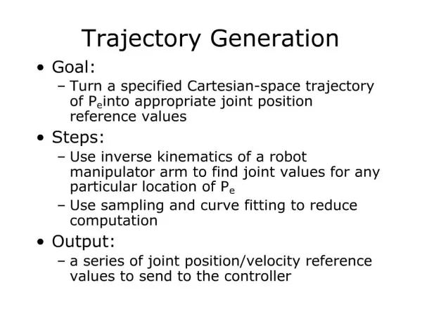
Trajectory Generation. Trajectory Generation – Problem Definition. Problem Given: Manipulator geometry, End Effector via point or Trajectory Compute: The trajectory of each joint such that the end effector move in space

E N D
Trajectory Generation Instructor: Jacob Rosen Advanced Robotic - MAE 263D - Department of Mechanical & Aerospace Engineering - UCLA
Trajectory Generation – Problem Definition Problem Given:Manipulator geometry, End Effector via point or Trajectory Compute: The trajectory of each joint such that the end effector move in space from point A to Point B Solution (Domains) • Joint space / Cartesian Space Definitions • Trajectory (Definition) - Time history of position, velocity, and acceleration for each DOF. • Trajectory Generation – Methods of computing a trajectory that describes the desired motion of a manipulator in a multidimensional space Instructor: Jacob Rosen Advanced Robotic - MAE 263D - Department of Mechanical & Aerospace Engineering - UCLA
Instructor: Jacob Rosen Advanced Robotic - MAE 263D - Department of Mechanical & Aerospace Engineering - UCLA
Trajectory Generation – Problem Definition • Human Machine interface (requirements) • Human - Specifying trajectories with simple description of the desired motion • Example – start / end points position and orientation of the end effectors • System - Designing the details of the trajectory • Example – Design the exact shape of the path, duration, joint velocity, etc. • Trajectory Representation • Representation of trajectory in the computer after they were planned • Trajectory Generation • Generation occurs at runtime (real time) where positions, velocities, and accelerations are computed. • Path update rate 60-2000 Hz Instructor: Jacob Rosen Advanced Robotic - MAE 263D - Department of Mechanical & Aerospace Engineering - UCLA
General Consideration • General approach for the motion of the manipulator • Specify the path as a motion of the tool frame {T} relative to the station frame {S}. Frame {S} may change it position in time (e.g. conveyer belt) • Advantages • Decouple the motion description from any particular robot, end effector, or workspace. • Modularity – Use the same path with: • Different robot • Different tool size Instructor: Jacob Rosen Advanced Robotic - MAE 263D - Department of Mechanical & Aerospace Engineering - UCLA
General Consideration • Basic Problem – Move the tool frame {T} from its initial position / orientation {T_initial} to the final position / orientation {T_final}. • Specific Description • Via Point – Intermediate points between the initial and the final end- effector locations that the end-effector mast go through and match it position and orientation along the trajectory. • Each via point is defined by a frame defining the position/orintataion of the tool with respect to the station frame • Path Points – includes all the via points along with the initial and final points • Point (Frame) – Every point on the trajectory is define by a frame (spatial description) Instructor: Jacob Rosen Advanced Robotic - MAE 263D - Department of Mechanical & Aerospace Engineering - UCLA
General Consideration • “Smooth” Path or Function • Continuous path / function with first and second derivatives. • Add constrains on the spatial and temporal qualities of the path between the via-points • Great verity of ways in which paths might be specified or planned. • Implications of non-smooth path • Increase wear in the mechanism (rough jerky movement) • Vibration – exciting resonances. Instructor: Jacob Rosen Advanced Robotic - MAE 263D - Department of Mechanical & Aerospace Engineering - UCLA
Joint Space Schemes • Joint space Schemes – Path shapes (in space and in time) are described in terms of functions in the joint space. • General process (Steps) given initial and target P/O • Select a path point or via point (desired position and orientation of the tool frame {T} with respect to the base frame {s}) • Convert each of the “via point” into a set of joint angles using the invers kinematics • Find a smooth function for each of the n joints that pass trough the via points, and end the goal point. Note 1: The time required to complete each segment is the same for each joint such that the all the joints will reach the via point at the same time. Thus resulting in the position and orientation of the frame {T} at the via point. Note 2: The joints move independently with only one time restriction (Note 1) Instructor: Jacob Rosen Advanced Robotic - MAE 263D - Department of Mechanical & Aerospace Engineering - UCLA
Joint Space Schemes – Cubic Polynomials • Define a function for each joint such that value at is the initial position of the joint and whose value at is the desire goal position of the joint • There are many smooth functions that may be used to interpolate the joint value. Instructor: Jacob Rosen Advanced Robotic - MAE 263D - Department of Mechanical & Aerospace Engineering - UCLA
Joint Space Schemes – Cubic Polynomials Problem - Define a function for each joint such that it value at is the initial position of the joint and at is the desired goal position of the joint Given - Constrains on What should be the order of the polynomial function to meet these constrains? Instructor: Jacob Rosen Advanced Robotic - MAE 263D - Department of Mechanical & Aerospace Engineering - UCLA
Joint Space Schemes – Cubic Polynomials • Solution - The four constraints can be satisfied by a polynomial of at least third degree • The joint velocity and acceleration • Combined with the four desired constraints yields four equations in four unknowns Instructor: Jacob Rosen Advanced Robotic - MAE 263D - Department of Mechanical & Aerospace Engineering - UCLA
Joint Space Schemes – Cubic Polynomials • Solving these equations for the we obtain Instructor: Jacob Rosen Advanced Robotic - MAE 263D - Department of Mechanical & Aerospace Engineering - UCLA
Joint Space Schemes – Cubic Polynomials • Example – A single-link robot with a rotary joint is motionless at degrees. It is desired to move the joint in a smooth manner to degrees in 3 seconds. Find the coefficient of the cubic polynomial that accomplish this motion and brings the manipulator to rest at the goal Instructor: Jacob Rosen Advanced Robotic - MAE 263D - Department of Mechanical & Aerospace Engineering - UCLA
Joint Space Schemes – Cubic Polynomials • The velocity profile of any cubic function is a parabola • The acceleration profile of any cubic function is linear Instructor: Jacob Rosen Advanced Robotic - MAE 263D - Department of Mechanical & Aerospace Engineering - UCLA
Joint Space Schemes – Cubic Polynomials – Via Points Previous Method - The manipulator comes to rest at each via point General Requirement - Pass through a point without stopping Problem - Define a function for each joint such that it value at is the initial position of the joint and at is the desire goal position of the joint Given - Constrains on such that the velocities at the via points are not zero but rather some known velocities Instructor: Jacob Rosen Advanced Robotic - MAE 263D - Department of Mechanical & Aerospace Engineering - UCLA
Joint Space Schemes – Cubic Polynomials – Via Points Solution - The four constraints can be satisfied by a polynomial Combined with the four desired constraints yields four equations in four unknowns Instructor: Jacob Rosen Advanced Robotic - MAE 263D - Department of Mechanical & Aerospace Engineering - UCLA
Joint Space Schemes – Cubic Polynomials – Via Points Solving these equations for the we obtain Given - velocities at each via point are Solution - Apply these equations for each segment of the trajectory. Instructor: Jacob Rosen Advanced Robotic - MAE 263D - Department of Mechanical & Aerospace Engineering - UCLA
Joint Space Schemes – Cubic Polynomials – Via Points • Specify the desired velocities at each segment: • User Definition – Desired Cartesian linear and angular velocity of the tool frame at each via point. • System Definition – The system automatically chooses the velocities (Cartesian or angular) automatically using a suitable heuristic method. • System Definition – The system automatically chooses the velocities (Cartesian or angular) to cause the acceleration at the via point to be continuous. Instructor: Jacob Rosen Advanced Robotic - MAE 263D - Department of Mechanical & Aerospace Engineering - UCLA
Joint Space Schemes – Cubic Polynomials – Via Points User Definition – Desired Cartesian linear and angular velocity of the tool frame at each via point. Mapping (Cartesian Space to Joint Space) - Cartesian velocities at the via point are “mapped” to desired joint rates by using the inverse Jacobian Singularity - If the manipulator is at a singular point at a particular via point then the user is not free to choose an arbitrarily velocity at this point. Difficult Instructor: Jacob Rosen Advanced Robotic - MAE 263D - Department of Mechanical & Aerospace Engineering - UCLA
Joint Space Schemes – Cubic Polynomials – Via Points 2. System Definition – The system automatically chooses the velocities (Cartesian or angular) using a suitable heuristic method given a trajectory . Heuristic method • Consider a path defined by via points • Connect the via points with straight lines • If the slope change sign • Set the velocity at the via point to be zero • If the slope have the same sign • Calculate the average between the to velocities at the via point. Instructor: Jacob Rosen Advanced Robotic - MAE 263D - Department of Mechanical & Aerospace Engineering - UCLA
Joint Space Schemes – Cubic Polynomials – Via Points System Definition – The system automatically chooses the velocities (Cartesian or angular) to cause the acceleration at the via point to be continuous. Spline - Enforcing the velocity and the acceleration to be continuous at the via point Instructor: Jacob Rosen Advanced Robotic - MAE 263D - Department of Mechanical & Aerospace Engineering - UCLA
Cubic Polynomials – Via Points – Example • Solve for the coefficients of two cubic functions that are connected in a two segment spline with a continuous acceleration at the intermediate via point. Instructor: Jacob Rosen Advanced Robotic - MAE 263D - Department of Mechanical & Aerospace Engineering - UCLA
Cubic Polynomials – Via Points – Example The joint angle velocity and acceleration for each segment (8 unknowns ) Instructor: Jacob Rosen Advanced Robotic - MAE 263D - Department of Mechanical & Aerospace Engineering - UCLA
Cubic Polynomials – Via Points – Example Position at the beginning and end of each segment Segment 1 Segment 2 Instructor: Jacob Rosen Advanced Robotic - MAE 263D - Department of Mechanical & Aerospace Engineering - UCLA
Cubic Polynomials – Via Points – Example Velocity at the beginning of the interval Velocity at the end of the interval Velocity at the mid point between the intervals Instructor: Jacob Rosen Advanced Robotic - MAE 263D - Department of Mechanical & Aerospace Engineering - UCLA
Cubic Polynomials – Via Points – Example Acceleration at the mid point between the intervals Solve 8 equations with 8 unknown Instructor: Jacob Rosen Advanced Robotic - MAE 263D - Department of Mechanical & Aerospace Engineering - UCLA
Cubic Polynomials – Via Points – Example Solution for the 8 equations Instructor: Jacob Rosen Advanced Robotic - MAE 263D - Department of Mechanical & Aerospace Engineering - UCLA
Joint Space Schemes – High Order Polynomials Problem - Define a function for each joint such that it value at is the time at the initial position is the time at the desired goal position Given - Constrains on the position velocity and acceleration at the beginning and the end of the path segment What should be the order of the polynomial function to meet these constrains? Instructor: Jacob Rosen Advanced Robotic - MAE 263D - Department of Mechanical & Aerospace Engineering - UCLA
Joint Space Schemes – High Order Polynomials Solution - The six constraints can be satisfied by a polynomial of at least fifth order Combined with the six desired constraints yields six equations with six unknowns Instructor: Jacob Rosen Advanced Robotic - MAE 263D - Department of Mechanical & Aerospace Engineering - UCLA
Joint Space Schemes – Cubic Polynomials Solving these equations for the we obtain Instructor: Jacob Rosen Advanced Robotic - MAE 263D - Department of Mechanical & Aerospace Engineering - UCLA
Joint Space Schemes – Linear Function With Parabolic Blend Instructor: Jacob Rosen Advanced Robotic - MAE 263D - Department of Mechanical & Aerospace Engineering - UCLA
Joint Space Schemes – Linear Function With Parabolic Blend Instructor: Jacob Rosen Advanced Robotic - MAE 263D - Department of Mechanical & Aerospace Engineering - UCLA
Joint Space Schemes – Linear Function With Parabolic Blend Instructor: Jacob Rosen Advanced Robotic - MAE 263D - Department of Mechanical & Aerospace Engineering - UCLA
Joint Space Schemes – Linear Function With Parabolic Blend Instructor: Jacob Rosen Advanced Robotic - MAE 263D - Department of Mechanical & Aerospace Engineering - UCLA
Joint Space Schemes – Linear Function With Parabolic Blend Instructor: Jacob Rosen Advanced Robotic - MAE 263D - Department of Mechanical & Aerospace Engineering - UCLA
Joint Space Schemes – Linear Function With Parabolic Blend Instructor: Jacob Rosen Advanced Robotic - MAE 263D - Department of Mechanical & Aerospace Engineering - UCLA
Cartesian Space Schemes – Introduction Joint Space Schemes Advantages – Path go through all the via and goal points Points can be specified by Cartesian frames. Disadvantages - End effector moves along a curved line (not a straight line - shortest distance). Path depends on the particular joint kinematics of the manipulator Instructor: Jacob Rosen Advanced Robotic - MAE 263D - Department of Mechanical & Aerospace Engineering - UCLA
Cartesian Space Schemes – Introduction Cartesian Space Scheme Advantage Most common path is straight line (shortest). Other shapes can also be used. Disadvantage Computationally expansive to execute – At run time the inverse kinematics needs to be solved at path update rate (60-2000 Hz) Instructor: Jacob Rosen Advanced Robotic - MAE 263D - Department of Mechanical & Aerospace Engineering - UCLA
Cartesian Space Scheme – Cartesian Straight Line • General Approach - Define the path (in the Cartesian space) as • straight lines (linear functions) • Parabolic lines (blends) Instructor: Jacob Rosen Advanced Robotic - MAE 263D - Department of Mechanical & Aerospace Engineering - UCLA
Cartesian Space Scheme – Cartesian Straight Line • General Approach (continue) • Every point along the path is defined by position and orientation of the end effector • End Effector Position – Vector – Easy interpolation • End Effector Ordination – Matrix – Impossible to interpolate (interpolating the individual elements of the matrix violate the requirements that all column of the matrix must be orthogonal) Instructor: Jacob Rosen Advanced Robotic - MAE 263D - Department of Mechanical & Aerospace Engineering - UCLA
Equivalent Angle – Axis Representation • Start with the frame coincident with a know frame {A}; then rotate frame {B} about a vector by an angle according to the right hand rule. • Equivalent Angle – Axis Representation • Vector is called the equivalent axis of a finite rotation. • The specification of requires two parameters since it length is always 1. • The angle specify the third parameter Instructor: Jacob Rosen Advanced Robotic - MAE 263D - Department of Mechanical & Aerospace Engineering - UCLA
Equivalent Angle – Axis Representation • Conversion 1 - Conversion for single angle axis representation to rotation matrix representation • Conversion 2 – Compute and given a rotation a matrix Instructor: Jacob Rosen Advanced Robotic - MAE 263D - Department of Mechanical & Aerospace Engineering - UCLA
Cartesian Space Scheme – Cartesian Straight Line • Combining the angle-axis representation of orientation with the 3x1 Cartesian position representation we have a 6x1 representation of Cartesian position and orientation. • Consider a via point specified relative to a station point frame as • Frame {A} specifies a via point • Position of the end effector given by • Orientation of the end effector given by Instructor: Jacob Rosen Advanced Robotic - MAE 263D - Department of Mechanical & Aerospace Engineering - UCLA
Cartesian Space Scheme – Cartesian Straight Line • Convert the rotation matrix into an angle axis representation • Use the symbol to represent 6x1 position and orientation • Where is formed by scaling the unite vector by the amount of rotation
Cartesian Space Scheme – Cartesian Straight Line • Process - For a given trajectory we describe a spline function that smoothly vary these six quantities from path point to path point as a function of time. • Linear Spline with parabolic bland • Path shape between via points will be linear • When via points are passed, the linear and angular velocity of the end effector are changed smoothly Instructor: Jacob Rosen Advanced Robotic - MAE 263D - Department of Mechanical & Aerospace Engineering - UCLA
Cartesian Space Scheme – Cartesian Straight Line • Complication – The angle-axis representation is not unique • In going from via point {A} to a via point {B}, the total amount of rotation should be minimized • Choose such that Instructor: Jacob Rosen Advanced Robotic - MAE 263D - Department of Mechanical & Aerospace Engineering - UCLA
Cartesian Space Scheme – Cartesian Straight Line • The splines are composed of linear and parabolic blend section • Constrain • The transition between the linear segment and the parabolic segment for all the DOF must take place at the same time. Instructor: Jacob Rosen Advanced Robotic - MAE 263D - Department of Mechanical & Aerospace Engineering - UCLA
Geometric Problems – Cartesian Paths • Problem Type 1 – Unreachable Intermediate Points • The initial and the final point are in the reachable workspace however some point along the path may be out of the workspace. • Solution • Joint space path – reachable • Cartesian straight Path – Unreachable Instructor: Jacob Rosen Advanced Robotic - MAE 263D - Department of Mechanical & Aerospace Engineering - UCLA
Geometric Problems – Cartesian Paths • Problem Type 2 – High Joint Rate Near Singularity. • In singularity the velocity of one or more joint approach infinity. • The velocity of the mechanism are upper bounded, approaching singularity results in the manipulator’s deviation form the desired path. • Solution • Slow down the velocity such that all the joint velocities will remain in their bounded velocities Instructor: Jacob Rosen Advanced Robotic - MAE 263D - Department of Mechanical & Aerospace Engineering - UCLA
Geometric Problems – Cartesian Paths • Problem Type 3 – Start and Goal reachable in different solutions • Joint limits may restrict the number of solutions that the manipulator may use given a goal point. • Solution • Switch between joint space (default) and Cartesian space trajectories (used only if needed) Instructor: Jacob Rosen Advanced Robotic - MAE 263D - Department of Mechanical & Aerospace Engineering - UCLA