Download
1 / 18
180 likes | 224 Views
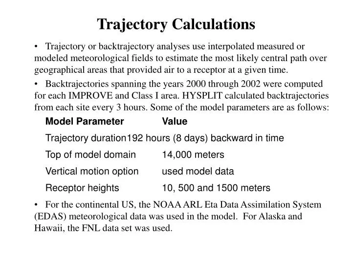
Trajectory Calculations. Trajectory or backtrajectory analyses use interpolated measured or modeled meteorological fields to estimate the most likely central path over geographical areas that provided air to a receptor at a given time.

E N D
Trajectory Calculations • Trajectory or backtrajectory analyses use interpolated measured or modeled meteorological fields to estimate the most likely central path over geographical areas that provided air to a receptor at a given time. • Backtrajectories spanning the years 2000 through 2002 were computed for each IMPROVE and Class I area. HYSPLIT calculated backtrajectories from each site every 3 hours. Some of the model parameters are as follows: Model ParameterValue Trajectory duration 192 hours (8 days) backward in time Top of model domain 14,000 meters Vertical motion option used model data Receptor heights 10, 500 and 1500 meters • For the continental US, the NOAA ARL Eta Data Assimilation System (EDAS) meteorological data was used in the model. For Alaska and Hawaii, the FNL data set was used.
Residence Time Maps • Residence time analysis computes the amount of time (e.g. hours) or percent of time the parcel is in a horizontal grid cell. In the figures presented below, residence time is shown as percent of total hours in each grid cell. • The domain of interest is divided into areas as one-degree latitude by one-degree longitude cells. • Overall and Monthly residence time maps, and residence time maps for the 20% worst and best visibility days, and 20% highest and lowest concentration days of individual aerosol chemical components (e.g. sulfate, nitrate, etc.) are created. • Conditional probability maps show the likelihood of having 20% worst visibility and 20% highest concentration of each aerosol chemical component occurring when air passed over each grid cell (The average would be 20%). Areas with high conditional probability indicate that when air passes over those grid cells, it is very likely to be associated with poor visibility at the receptor.
Limitations • The meteorological input fields typically used represent large-scale flows and cannot accurately represent local to mesoscale flows such as topographically influenced flow, nocturnal jets, and seabreeze/landbreeze. • It some cases systematic biases may occur that could lead to invalid conclusions regarding source-receptor relationships.
Residence Time Maps at Grand Canyon August January
Residence Time Maps at Grand Canyon (continue) Worst 20% Days Best 20% Days
Residence Time Maps at Grand Canyon (continue) 20% worst OC 20% worst sulfate
Residence Time Maps at Grand Canyon (continue) Difference (top left) and ratio (bottom right) of normalized residence time in 20% worst sulfate days and all days in 2000-2002 (possible important source regions are shown up as blue in the maps)
Causes of Haze Assessment Transport Regression Modeling • To explain an air quality parameter (dependent variable) using the numbers of back-trajectory endpoints in arbitrarily selected source regions (independent variables) using multiple linear regression • Approach for grouping the source regions • Divide the state containing the monitoring site into quadrants (i.e. NE, SE, SW, & NW) with the origin at the monitoring sites. • Have every state bordering the state containing the monitoring site as a separate source region (i.e. neighboring states). • Group all other states beyond the bordering states into four quadrants. The boundaries will be the same regardless of the monitoring site, except that neighboring states are excluded. • Include Mexico, Canada, Pacific Ocean, Gulf of Mexico, and Atlantic Oceans as separate source regions. • This gives a total of from 9 to 19 source regions in the western contiguous states. • For the states of Alaska & Hawaii, divide the states into quadrants, and everything outside of the states into quadrants for a total of 8 source regions
Transport Regression Modeling Results • Air Quality Parameter (e.g. Sulfate Concentration) = (Correlation Coefficient * Residence Time in the Source Region)
Contribution to Sulfate at Grand Canyon Based on Transport Regression Modeling 2.9% 0.2% 19% 3.1%
Comparison Between Measured and Calculated Sulfur Concentrations (ng/m3) at Grand Canyon
Comparison of Regression Modeling Results at Grand Canyon Using Residence Time at 10m, 500m, 1500m and All Three Heights
Comparison of Percentage Contributions to Aerosol Extinction Coefficient (Bep) and Sulfur Concentration at Grand Canyon
Percentage Contribution to Sulfate at Badlands Based on Transport Regression Modeling 0.3 6.1 -3.5 22.7 8.1 10.5 -0.4 11.7 5.7 5.5 -0.1 -0.6 0.8 12.3 11.4 -0.6 0.3 3.1 6.8
Percentage Contribution to Sulfate at Craters of the Moon Based on Transport Regression Modeling 10.3 1.6 11 7.0 -0.4 3.1 3.9 27.5 2.1 0.5 -0.3 6.8 5.7 2.3 -0.03 18.1 0.7 -0.2
Comparison of Percentage Contributions to Bep, Nitrate, Sulfur and OC Concentrations at Crates of the Moon
Comparison of Percentage Contributions to Bep, Sulfur and Nitrate Concentrations at Joshua Tree Wilderness Area
Percentage Contribution to Sulfate at Mount Rainer National Park Based on Transport Regression Modeling 0.1 2.3 35 -0.4 17 0 -0.1 7.2 -5.4 0.6 -0.3 44 -0.4 0.3