Trajectory Generation

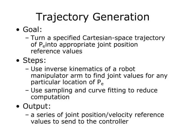
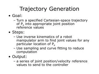
1. Trajectory Generation • Goal: • Turn a specified Cartesian-space trajectory of Pe into appropriate joint position reference values • Steps: • Use inverse kinematics of a robot manipulator arm to find joint values for any particular location of Pe • Use sampling and curve fitting to reduce computation • Output: • a series of joint position/velocity reference values to send to the controller

2. Obtain function for workspace path Sample function to get discrete joint pts Apply IK & Jacobian calculations Fit function to joint points Sample to get discrete reference points C D D C D 5 Step Process for Trajectory Generation C=continuous D=discrete

3. Step One: Continuous Fcn • Obtain an analytic function to describe motion with respect to the base frame • Obtain rate of change of location

4. Step 2: Sample • Sample the trajectory to obtain a finite number, m, of sample points on the continuous trajectory: • Sample rate of change

5. Step 3: IK & J • (a) Use inverse kinematics to convert each Cartesian trajectory sample point vector, into a corresponding joint space vector, • Handle multiple solutions, admissibility, etc.

6. Step 3: IK & J • (b) Use the inverse Jacobian relation to convert each velocity vector, into a corresponding joint speed vector, • Handle singular configurations

7. Step 4: Fit Continuous Curve to Joint Points • Use the sequence of vectors and i=1,…,m to generate continuous expressions for each joint and j=1,…,dof which pass through or sufficiently near to each of joint space sample points, and rate of change sample points, to produce continuous joint space trajectories for each joint.

8. Step 4: Fit Continuous Curve to Joint Points Spline or Polynomial Fit & derivatives:

9. Step 4: Fit Continuous Curve to Joint Points Let’s look at fitting a curve to one interval

10. Step 4. Fit Continuous Curve to Joint Points • Fit a continuous function, q(t) to the points: • Time info – from original sampling • For now use notation (get rid of subscripts i and i+1): t=t0 t=tf

11. Step 4. Fit Continuous Curve to Joint Points • Splines, polynomials,… • To match position, velocity and acceleration at end points use a quintic polynomial (6 parameters to match the 6 unknowns):

12. Step 4. Fit Continuous Curve to Joint Points • Note: To match only position and velocity at end points use a cubic polynomial (4 parameters to match the 4 unknowns):

13. Step 4. Fit Continuous Curve to Joint Points • Use endpoints and time values in quintic polynomial (6 linear equations, 6 unknowns)

14. Step 4. Fit Continuous Curve to Joint Points • In matrix form:

15. Step 4. Fit Continuous Curve to Joint Points • In matrix form:

16. Step 4: Computational Thoughts • Need to perform fit for each joint but… on each TIME interval, this matrix is the same for each joint – compute inverse only once

17. Step 4: Fit Continuous Curve to Joint Points ….. one for each time interval (i, i+1) Piecewise polynomials: one polynomial for each joint for each timte interval (and we can easily take derivatives)

18. Step 5: Sample Joint Curve • Sample each continuous joint trajectory to generate a sequence of discrete reference values for each joint, where ttotal/N is the sampling period used. Sample

19. Step 5: Sample Joint Curve • Sample joint speeds. Sample

20. Workspace path function Sample -- discrete joint pts Apply IK & Jacobian calculations Joint function Sample -- discrete reference points C m pts m pts C N pts 5 Step Process for Trajectory Generation m ~ 10 N ~ 1000+ Note: N >> m

21. Example: Linear Motion • Step One: Express line as continuous function (i.e. parameterize by time): • x(t), y(t), f(t) • Suppose we specify the line y= mx +b • Want to move along line with constant speed, v

22. Parameterize the Line • Equation of line • Differentiate • Velocity vector • Substitute

23. Parameterize the Line • Velocity • Speed (magnitude) • Solve (pick appropriate sign)

24. Parameterize the Line • Velocity,

25. Sample Continuous Path Fcn • Use M samples for total time, ttotal time

26. Example Line • Let’s take a 2-link planar arm with • Link lengths: l1 = 4, l2 = 3 m • Line y= - x + l1+l2/4 or y=-x +4.75 with speed, v = 3m/s • Start point = (0, l1 + l2 /4)=(0,4.75) • endpoint = (l1 + l2 /4,0)=(4.75,0) • constant speed • Note, in practice, speed usually follows a trapezoidal profile with acceleration/deceleration at start/end of the motion

27. Example Line • Using our 2-link planar data the path has • And for constant speed will take

28. Example Line • We will use M=9 sample points • And for constant speed we will have

30. Step 3: IK & Jacobian • inverse kinematics: • where

31. Step 3: IK & Jacobian • Jacobian relationship:

32. Step 3: Discrete joint values

33. Step 3: Discrete Joint Velocity Values

34. Step 4: Fit Cubic To Positions/Speeds rmse = 0.014 rad ~ 1 deg

35. Curve Fitting Comments • Typically, a single cubic is not sufficient for the entire motion • A quintic polynomial can fit position, velocity and accelerations of end-points • What are the implications of fitting only position/velocity?

36. Reference Positions with 0.02s timesteps (sample cubic function)

38. CONS Actual robot position is sometimes unclear, particularly in presence of known obstacles PROS Actual control of the robot occurs in joint space Simpler to plan trajectories in real-time; less computation No problem with singularities Cartesian vs. Joint space

39. CONS Need Inverse kinematics (can be multi-valued) Smooth trajectory in Cartesian space may not map to continuous joint space trajectory Joint limits may prevent position from being realized End-effector paths may not be safe for rest of manipulator computational demand and analytic complexity PROS We usually desire a Cartesian path. Easy to visualize the trajectory Occurs in many robotic activities Shortest Euclidean path Straight line path minimizes inertial forces Cartesian trajectory can be robot independent Cartesian vs. Joint space

41. Path not in workspace Start & goal in different solution branches May need to flip between configurations