Download

1 / 47
470 likes | 573 Views
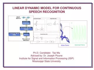
Pronunciation Modeling for Large Vocabulary Continuous Speech Recognition. Michael Picheny IBM TJ Watson Research Center Yorktown Heights, NY 10598. The statistical approach to speech recognition. W is a sequence of words, W* is the best sequence. X is a sequence of acoustic features.

E N D
Pronunciation Modeling for Large Vocabulary ContinuousSpeech Recognition Michael Picheny IBM TJ Watson Research Center Yorktown Heights, NY 10598
The statistical approach to speech recognition • W is a sequence of words, W* is the best sequence. • X is a sequence of acoustic features. • is a set of model parameters.
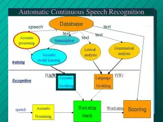
Automatic speech recognition – Architecture audio words feature extraction search acoustic model language model acoustic model language model
0.2 0.8 0.9 0.1 0.9 0.1 0.2 0.8 1 2 Hidden Markov Model • The state sequence is hidden. Unlike Markov Models, the state sequence cannot be uniquely deduced from the output sequence. • In speech, the underlying states can be, say the identities of the sounds generating the features. These are hidden – they are not uniquely deduced from the output features. We already mentioned that speech has memory. A process which has memory and hidden states implies HMM. 0.8 0.9 0.1 0.2
Three problems of general interest for an HMM 3 problems need to be solved before we can use HMM’s: • 1. Given an observed output sequence X=x1x2..xT , compute Pq(X) for a given model q • 2. Given X, find the most likely state sequence (Viterbi algorithm) • 3. Estimate the parameters of the model. (training) These problems are easy to solve for a state-observable Markov model. More complicated for an HMM because we need to consider all possible state sequences.
How do we use HMMs to model words? • Simplest idea: whole word model • For each word in the vocabulary, decide on a topology (states and transitions) • Often the number of states in the model is chosen to be proportional to the number of phonemes in the word • Train the observation and transition parameters for a given word using examples of that word in the training data (Recall problem 3 associated with Hidden Markov Models) • Good domain for this approach: digits
Example topologies: Digits • Vocabulary consists of {“zero”, “oh”, “one”, “two”, “three”, “four”, “five”, “six”, “seven”, “eight”, “nine”} • The “longer” the word the more states needed in the HMM • Must allow for different durations – use self loops and skip arcs • Models look like: • “zero” • “oh” 8 4 7 3 6 2 5 1 10 9
14 13 16 12 15 11 • “one” • “two” • “three” • “four” • “five” 20 19 18 17 24 23 26 22 25 21 30 29 32 28 31 27 36 35 38 34 37 33
42 41 • “six” • “seven” • “eight” • “nine” 44 40 43 39 46 45 50 49 52 51 48 47 54 53 56 55 60 59 58 57 64 63 66 62 65 61
41 42 39 40 43 44 45 46 49 50 52 51 48 47 54 53 56 55 59 60 57 58 63 64 62 65 66 61 4 7 8 3 6 1 2 5 How to represent any sequence of digits? 9 10 13 14 12 15 16 11 19 20 18 17 23 24 22 25 26 21 29 30 28 31 32 27 36 35 38 33 34 37
Whole-word model limitations • The whole-word model suffers from two main problems • 1. Cannot model unseen words. In fact, we need several samples of each word to train the models properly. Cannot share data among models – data sparseness problem. • 2. The number of parameters in the system is proportional to the vocabulary size. • Thus, whole-word models are best on small vocabulary tasks.
Subword Units • To reduce the number of parameters, we can compose word models from sub-word units. • These units can be shared among words. Examples include: UnitsApproximate number • Phones 50 • Diphones 2000 • Triphones 10,000 • Syllables 5,000 • Each unit is small • The number of parameters is proportional to the number of units (not the number of words in the vocabulary as in whole-word models.)
Phonetic Models • We represent each word as a sequence of phonemes. This representation is the “baseform” for the word. BANDS B AE N D Z • Some words need more than one baseform THE DH UH DH IY
Baseform Dictionary • To determine the pronunciation of each word, we look it up in a dictionary • Each word may have several possible pronunciations • Every word in our training script and test vocabulary must be in the dictionary • The dictionary is generally written by hand • Prone to errors and inconsistencies 2nd looks wrong AA K .. is missing acapulco | AE K AX P AH L K OW acapulco | AE K AX P UH K OW accelerator | AX K S EH L AX R EY DX ER accelerator | IX K S EH L AX R EY DX ER acceleration | AX K S EH L AX R EY SH IX N acceleration | AE K S EH L AX R EY SH IX N accent | AE K S EH N T accept | AX K S EH P T acceptable | AX K S EH P T AX B AX L access | AE K S EH S accessory | AX K S EH S AX R IY accessory | EH K S EH S AX R IY Shouldn’t the choices For the 1st phoneme be the Same for these 2 words? Don’t these words All start the same?
Phonetic Models, cont’d • We can allow for phonological variation by representing baseforms as graphs acapulco AE K AX P AH L K OW acapulco AA K AX P UH K OW L AH AE OW P K AX K AA UH
Phonetic Models, cont’d • Now, construct a Markov model for each phone. • Examples: p(length) length
Embedding • Replace each phone by its Markov model to get a word model • n.b. The model for each phone will have different parameter values L AH AE OW P K AX K AA UH
Reducing Parameters by Tying • Consider the three-state model • Note that • t1 and t2 correspond to the beginning of the phone • t3 and t4 correspond to the middle of the phone • t5 and t6 correspond to the end of the phone • If we force the output distributions for each member of those pairs to be the same, then the training data requirements are reduced. t5 t3 t1 t6 t2 t4
Tying • A set of arcs in a Markov model are tied to one another if they are constrained to have identical output distributions. • Similarly, states are tied if they have identical transition probabilities. • Tying can be done in various ways
Implicit Tying • Consider phone-based models for the digits vocabulary 0 Z IY R OW 1 W AA N 2 T UW 3 TH R IY 4 F AO R 5 F AY V 6 S IH K S 7 S EH V AX N 8 EY T 9 N AY N • Training samples of “0” will also affect models for “3” and “4” • Useful in large vocabulary systems where the number of words is much greater than the number of phones.
Explicit Tying Example: 6 non-null arcs, but only 3 different output distributions because of tying Number of model parameters is reduced Tying saves storage because only one copy of each distribution is saved Fewer parameters mean less training data needed e m b e b m
Variations in realizations of phonemes • The broad units, phonemes, have variants known as allophones Example: In English p and ph (un-aspirated and aspirated p) Exercise: Put your hand in front of your mouth and pronounce “spin” and then “pin.” Note that the p in “pin” has a puff of air, while the p in “spin” does not. • Articulators have inertia, thus the pronunciation of a phoneme is influenced by surrounding phonemes. This is known as co-articulation Example: Consider k and g in different contexts In “key” and “geese” the whole body of the tongue has to be pulled up to make the vowel Closure of the k moves forward compared to “caw” and “gauze” Phonemes have canonical articulator target positions that may or may not be reached in a particular utterance.
Allophones • In our speech recognition system, we typically have about 50 allophones per phoneme. • Older techniques (“tri-phones”) tried to enumerate by hand the set of allophones for each phoneme. • We currently use automatic methods to identify the allophones of a phoneme. • One way is a class of statistical models known as decision trees • Classic text: L. Breiman et al. Classification and Regression Trees. Wadsworth & Brooks. Monterey, California. 1984.
Decision Trees • We would like to find equivalence classes among our training samples • The purpose of a decision tree is to map conditions (such as phonetic contexts) into equivalence classes • The goal in constructing a decision tree is to create good equivalence classes
Decision Tree Construction • 1. Find the best question for partitioning the data at a given node into 2 equivalence classes. • 2. Repeat step 1 recursively on each child node. • 3. Stop when there is insufficient data to continue or when the best question is not sufficiently helpful.
Decision Tree Construction – Fundamental Operation • There is only 1 fundamental operation in tree construction: Find the best question for partitioning a subset of the data into two smaller subsets. i.e. Take an equivalence class and split it into 2 more-specific classes.
Decision Tree Greediness • Tree construction proceeds from the top down – from root to leaf. • Each split is intended to be locally optimal. • Constructing a tree in this “greedy” fashion usually leads to a good tree, but probably not globally optimal. • Finding the globally optimal tree is an NP-complete problem: it is not practical (and not clear it matters)
Pre-determined Questions • The easiest way to construct a decision tree is to create in advance a list of possible questions for each variable. • Finding the best question at any given node consists of subjecting all relevant variables to each of the questions, and picking the best combination of variable and question. • In acoustic modeling, we typically ask about 10 variables: the 5 phones to the left of the current phone and the 5 phones to the right of the current phone. Since these variables all span the same alphabet (phone alphabet) only one list of questions. • Each question on this list consists of a subset of the phonetic phone alphabet.
Sample Questions {P} {T} {K} {B} {D} {G} {P,T,K} {B,D,G} {P,T,K,B,D,G}
Simple Binary Question • A simple binary question consists of a single Boolean condition, and no Boolean operators. • X1 c S1? Is a simple question. • (( X1 c S1) && ( X2 c S2))? Is not a simple question. • Topologically, a simple question looks like: xcS? N Y
Complex Binary Question • A complex binary question has precisely 2 outcomes (yes, no) but has more than 1 Boolean condition and at least 1 Boolean operator. • (( X1 c S1) && ( X2 c S2))? Is a complex question. • Topologically this question can be shown as: • All complex questions can be represented as binary trees with terminal nodes tied to produce 2 outcomes. x1cS1? N 2 Outcomes: ( X1c S1) 3 ( X2c S2) ( X1c S1) 3 ( X2c S2) =( X1c S1) 4 ( X2c S2) Y x2cS2? 1 2 N Y 1 2
Configurations Currently Used • All decision trees currently used in speech recognition use: a pre-determined set of simple, binary questions on discrete variables.
Tree Construction Overview • Let x1 … xn denote n discrete variables whose values may be asked about. Let Qij denote the jth pre-determined question for xi. • Starting at the root, try splitting each node into 2 sub-nodes: • 1. For each variable xi evaluate questions Qi1, Qi2, … and let Q’i denote the best. • 2. Find the best pair xi,Q’i and denote it x’,Q’. • 3. If Q’ is not sufficiently helpful, make the current node a leaf. • 4. Otherwise, split the current node into 2 new sub-nodes according to the answer of question Q’ on variable x’. • Stop when all nodes are either too small to split further or have been marked as leaves.
Question Evaluation • The best question at a node is the question which maximizes the likelihood of the training data at that node after applying the question. • Goal: Find Q such that L(datal|ml,Sl) x L(datar|mr,Sr) is maximized. Parent node: Model as a single Gaussian N(mp,Sp) Compute likelihood L(datap|mp,Sp) Q? N Y Left child node: Model as a single Gaussian N(ml,Sl) Compute likelihood L(datal|ml,Sl) Right child node: Model as a single Gaussian N(mr,Sr) Compute likelihood L(datar|mr,Sr)
Question Evaluation, cont’d • Let x1,x2,…xN be a sample of feature x, in which outcome ai occurs ci times. • Let Q be a question which partitions this sample into left and right sub-samples of size nl and nr, respectively. • Let cil, cir denote the frequency of ai in the left and right sub-samples. • The best question Q for feature x is the one which maximizes the conditional likelihood of the sample given Q, or, equivalently, maximizes the conditional log likelihood of the sample.
Best Question: Context-Dependent Prototypes • For context-dependent prototypes, we use a decision tree for each arc in the Markov model. • At each leaf of the tree is a continuous distribution which serves as a context-dependent model of the acoustic vectors associated with the arc. • The distributions and the tree are created from acoustic feature vectors aligned with the arc. • We grow the tree so as to maximize the likelihood of the training data (as always), but now the training data are real-valued vectors. • We estimate the likelihood of the acoustic vectors during tree construction using a diagonal Gaussian model. • When tree construction is complete, we replace the diagonal Gaussian models at the leaves by more accurate models to serve as the final prototypes. Typically we use mixtures of diagonal Gaussians.
Diagonal Gaussian Likelihood • Let Y=y1y2yn be a sample of independent p-dimensional acoustic vectors arising from a diagonal Gaussian distribution with mean m and variances s2. Then • The maximum likelihood estimates of m and s2 are: • Hence, an estimate of log L(Y) is
Diagonal Gaussian Likelihood • Now, • Hence
Diagonal Gaussian Splits • Let Q be a question which partitions Y into left and right sub-samples Yl and Yr, of size nl and nr. • The best question is the one which maximizes logL(Yl)+logL(Yr) • Using a diagonal Gaussian model Common to all splits
Diagonal Gaussian Splits, cont’d • Thus, the best question Q minimizes: • Where • DQ involves little more than summing vector elements and their squares.
How Big a Tree? • CART suggests cross-validation • Measure performance on a held-out data set • Choose the tree size that maximizes the likelihood of the held-out data • In practice, simple heuristics seem to work well • A decision tree is fully grown when no terminal node can be split • Reasons for not splitting a node include: • Insufficient data for accurate question evaluation • Best question was not very helpful / did not improve the likelihood significantly • Cannot cope with any more nodes due to CPU/memory limitations
Putting it all together Given a word sequence, we can construct the corresponding Markov model by: • Re-writing word string as a sequence of phonemes • Concatenating phonetic models • Using the appropriate tree for each arc to determine which alloarc (leaf) is to be used in that context
Example The rain in Spain falls …. Look these words up in the dictionary to get: DH AX | R EY N | IX N | S P EY N | F AA L Z | … Rewrite phones as states according to phonetic model DH1 DH2 DH3 AX1 AX2 AX3 R1 R2 R3 EY1 EY2 EY3 … Using phonetic context, descend decision tree to find leaf sequences DH1_5 DH2_27 DH3_14 AX1_53 AX2_37 AX3_11 R1_42 R2_46 …. Use the Gaussian mixture model for the appropriate leaf as the observation probabilities for each state in the Hidden Markov Model.
Recognition Performance • From Julian Odell’s PhD Thesis (1995) (Cambridge) • Resource Management (1K vocabulary task)