Download

1 / 31
310 likes | 464 Views
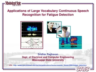
Applications of Large Vocabulary Continuous Speech Recognition for Fatigue Detection. Sridhar Raghavan Dept. of Electrical and Computer Engineering Mississippi State University URL: http://www.cavs.msstate.edu/hse/ies/publications/books/msstate_theses/2006/fatigue_detection/. Abstract.

E N D
Applications of Large Vocabulary Continuous Speech Recognition for Fatigue Detection Sridhar Raghavan Dept. of Electrical and Computer Engineering Mississippi State University URL: http://www.cavs.msstate.edu/hse/ies/publications/books/msstate_theses/2006/fatigue_detection/
Abstract • Goal of the thesis: To automate the task of fatigue detection using voice. • Problem statement: Determine a suitable technique to enable automatic fatigue detection using voice. Also make the system robust to out-of-vocabulary words which directly influence fatigue detection performance. • Hypothesis: An LVCSR system can be used for detecting fatigue from voice. • Results: Using confidence measures the robustness of the fatigue detection system to out-of-vocabulary words improved by 20%.
Motivation • Applications of speech recognition have grown from simple speech to text • conversion to other more challenging tasks. An ASR system can be used as a • core and various applications can be built using the same technology. This • thesis explores the application of speech recognition to the task of • fatigue detection from voice. The ISIP ASR toolkit was used as the core speech • engine for this thesis. Automobile Telematics Speech Therapy systems Speech Recognition Core Speech Engine Speaker Verification Focus of this thesis Fatigue Detection word Spotting Automatic Call routing Automatic Language Detection
Signs of Fatigue in Human Speech • Creare Inc. provided voice data recorded from subjects who were • induced with fatigue by sleep depravation. The spectrograms of a subject • before and after fatigue induction is shown below. • Non-fatigued speaker saying “papa” • Fatigued speaker saying “papa”
Changes in Human Voice Production System due to Fatigue • From literature it is known that fatigue causes temporal and spectral variations • in the speech signal. The spectral variation can be attributed to a change in the • human sound production system, while the temporal variation is controlled by • the brain and its explanation is beyond the scope of this thesis. • Effects on human sound production system: • Yielding walls: The vocal tract walls are not rigid and hence it is known that an increase in the vibration of the walls of the vocal tract causes a slight increase in the lower order formants. • Viscosity and thermal loss: It is the friction between air and walls of the vocal tract. This loss causes a slight upward shift on the formant frequencies that exist beyond 3-4 kHz. • Lip radiation: For an ideal vocal tract model the lip radiation loss is ignored, but it is known from literature that the lip radiation loss causes a slight decrease in the formants. This effect is more pronounced for higher order formants.
Fatigue detection using a Speaker Verification System • Speaker Verification: A speaker verification system can be used to model the • long term speech characteristics of a speaker. The system builds a model for • each individual speaker. Verification is performed by computing a likelihood • (likelihood is defined as the conditional probability of the acoustic data • given the speaker model). • Fatigue detection using the speaker verification system was conducted as • follows: • Models were trained on data that was collected during the initial stage of the recordings. • These models were used for testing. There were six recording stages evenly spread over a duration of thirty six hours.
Result from Pilot Speaker verification Experiments Active Speaker Model MFCCs Active or fatigued utterance from the speaker Output Input Speaker Verification Observation: No significant difference in the likelihood scores was observed. Distribution of the likelihood scores of fatigued and non-fatigued speakers • One probable reason for poor performance is that not all sounds in human • speech are affected by fatigue in the same manner.
Effect of Fatigue on Different Phonemes • Greeley, et al. found that not all phonemes are affected equally due to fatigue. • Certain phonemes showed more variations due to fatigue than others. Certain sounds showed more variations due to fatigue than others
Fatigue Detection using a Word Spotter • Word Spotting system: A word spotting system determines the presence of • words of interest in a speech file. Such a system was built using the ISIP ASR • system as follows: • Labeled training data was used to train the acoustic models. • A garbage model is built by labeling all the words in the transcription by the same token. The garbage model will be used as a substitute for any word other than the keyword in the final hypothesis. • The grammar of the recognizer was changed based on what words had to be spotted. Measure of fatigue Fatigue Detection Input utterance Word Spotter spotted word alignment Loop grammar The problem with this system was that it generated a high percentage of false hypothesis and this affected fatigue detection performance.
Speech signal ASR System Output Hypothesis Feature Extraction Fatigue Detection System Fatigue prediction output • An LVCSR Approach to Detect Fatigue • An ASR system trained on the Creare data provided reasonably accurate phonetic alignments. A WER of 11% was obtained. These alignments were used by the fatigue detection software to grab the MFCC vectors corresponding to specific sounds. • Advantage of using this approach is that: • 1. Unlike speaker verification technique this approach does not require fatigue • dependent data for training the ASR system. • 2. The grammar of the ASR is fixed unlike the word spotting technique. • But the problem of false alarms still exists, especially when there are out-of • -vocabulary words, and this problem is tackled by the use of confidence • measures.
Generating a Baseline ASR System Model selection experiments on FAA data Grammar tuning experiments on Phase II data using 16-mixture Cross-word triphones Mixture selection experiments on FAA data • Phase II data: This data was recorded during a three day military exercise using a PDA (Personal Digital Assistant). The data was very noisy and contained lot of disfluencies. There were 8 fixed phrases and one spontaneous phrase for each of the 21 speakers. • FAA data: This consisted of 30 words spoken in a studio environment over a three day period. The speakers read fixed text.
Results from state-tying experiments Closed loop state tying experiments • The performance of the system was improved further by tuning the state tying parameters. This was possible since cross-word triphone models were used as the fundamental acoustic model. Open loop state tying experiments • It was observed that the WER improved by increasing the number of states, but made the model specific to the training data. Hence an optimum value was chosen by observing the WER on open loop experiments.
Problem due to False Alarms • The output of an ASR system had some errors. The errors are classified as: substitutions, insertions and deletions. • The performance of the fatigue prediction system relied on the accuracy of the phonetic alignment. • It did not matter if the ASR miss-recognized the required words, but it did matter when there were false alarms. Reference Transcription KEEP THE POT INSIDE THE OVEN AND WAIT FOR FIFTEEN MINUTES. ASR’s Output HEAT THE POT INSIDE THE OPENAND POT FOR FIFTEEN MINUTES. Not a major problem since it will not be considered for fatigue analysis in any case Correct hypothesis, hence no problem and its alignments will be used for fatigue detection Very serious problem since a totally different MFCC vector set corresponding to the word “wait” will be analyzed assuming it is the word “pot”
Using Confidence Measures • By using confidence metric we could prune away less likely words that constituted false alarms. • The first choice for a confidence metric was the likelihood or the acoustic score of every word in the hypotheses. • Observation of the likelihood scores revealed that there was no clear trend that could be useful for pattern classification. • An example of such an observation is shown below
Word Posteriors as Confidence Measures • Word posteriors can be defined as “the sum of the posterior probabilities of all • word graph paths of which the word is a part”. • Word posteriors can be computed in two ways: • N-Best list • Word graphs • In this thesis the word posteriors were computed from word graphs as they are • much better representation of the search space than N-Best lists. Example of a word graph
Computing Word Posteriors from Word Graphs • Restating the word posterior definition for clarity: • Word posteriors can be defined as “the sum of the posterior probabilities of all • word graph paths of which the word is a part”. • What does this mean mathematically?
Computing Word Posteriors from Word Graphs We cannot compute the posterior probability directly, so we decompose it into likelihood and priors using Baye’s rule. N There are 6 different ways to reach the node N and 2 different ways to leave N, so we need to obtain the forward probability as well as the backward probability to determine the probability of passing through the node N, and this is where the forward-backward algorithm comes into picture. The numerator is computed using the forward backward algorithm. The denominator term is simply the by product of the forward-backward algorithm.
quest 1/6 a sense 1/6 the 1/6 Sil 1/6 is 2/6 1/6 guest sentence Sil 3/6 2/6 1/6 5/6 Sil This 2/6 4/6 is 3/6 4/6 3/6 the Sil sentence 2/6 this 1/6 is test a 4/6 4/6 a • Computing Word Posteriors from Word Graphs A Toy Example The values on the links are the likelihoods. Some nodes are outlined with red to signify that they occur at the same time instant.
Computing Word Posteriors from Word Graphs A forward-backward type algorithm will be used for determining the link probability. Computing alphas or the forward probability: Step 1: Initialization In a conventional HMM forward-backward algorithm we would perform the following: A slightly modified version of the above equation will be used on a word graph. The emission probability will be the acoustic score .
Computing Word Posteriors from Word Graphs The α for the first node is 1: Step 2: Induction The alpha values computed in the previous step are used to compute the alphas for the succeeding nodes. Note: Unlike in HMMs where we move from left to right at fixed intervals of time, over here we move from one node to the next based on node indices which are time aligned.
Computing Word Posteriors from Word Graphs Let us see the computation of the alphas from node 2, the alpha for node 1 was initialized as 1 in the previous step during initialization. Node 2: α=1.675E-05 α =0.005025 is 4 Node 3: α =1 3/6 2/6 Sil 1 4/6 3 3/6 3/6 Sil Node 4: this 2 α =0.005 The alpha calculation continues in this manner for all the remaining nodes.
Computing Word Posteriors from Word Graphs Once the alphas are computed using the forward algorithm, the betas are computed using the backward algorithm. The backward algorithm is similar to the forward algorithm, but the computation starts from the last node and proceed from right to left. Step 1 : Initialization Step 2: Induction
Computing Word Posteriors from Word Graphs Computation of the beta values from node 14 and backwards. Node 14: β=1.66E-5 β=0.001667 1/6 sense 14 1/6 Sil 1/6 11 sentence Sil Node 13: 5/6 13 15 4/6 β=1 sentence β=0.00833 12 Node 12: β=5.55E-5
Computing Word Posteriors from Word Graphs Node 11: In a similar manner we obtain the beta values for all the nodes till node 1. The alpha for the last node should be the same as the beta at the first node. The link probability is simply the product of the alpha and beta in its preceding and succeeding nodes. Note that this value is not normalized. It was normalized by dividing it with the sum of the probability of all paths through the word graph. The confidence measure was further strengthened by summing up the link probabilities of all similar words occurring within a particular time frame.
α=1.2923E-15 β=1.667E-03 α=7.751E-13 β=1.66E-05 α=1.675E-05 β=1.536E-13 α =5.025E-03 β=5.740E-14 quest 1/6 a sense 14 1/6 the 1/6 Sil 8 1/6 α =1 β=2.88E-16 is 2/6 4 1/6 guest 11 sentence Sil 3/6 2/6 1/6 5/6 Sil 6 This 2/6 1 4/6 13 15 3 is 9 4/6 3/6 α=1.861E-10 β=2.766E-8 α=2.88E-16 β=1 3/6 the Sil sentence 5 α=3.438E-14 β=8.33E-03 2/6 this 1/6 α=3.35E-5 β=8.537E-12 is test 2 a 4/6 4/6 12 α =5e-03 β=2.87E-16 7 10 α=4.964E-12 β=5.55E-05 α=7.446E-10 β=3.7E-07 α=1.117E-7 β=2.512E-9 • Word graph showing the computed alphas and betas This word graph shows every node with its corresponding alpha and beta computed. α=1.675E-7 β=4.61E-11 α=2.79E-10 β=2.766E-8 In this example the probability of occurrence of any word is fixed as it is a loop grammar and any word can follow any other word. Using a statistical language model should further strengthen the posterior scores.
quest p=-4.8978 13 p=-1.0986 p=-4.7156 p=-3.6169 p=-3.6169 sense p=--4.8978 7 is 3 the a 10 p=-3.2884 Sil p=-0.4051 guest Sil sentence 5 p=-0.0086 Sil 0 p=-4.0224 12 14 2 is p=-3.604 This 8 p=-0.0459 p=-0.0075 the Sil 4 p=-1.0982 sentence p=-0.0273 this p=-4.0224 is 1 test a 11 6 9 p=-0.0459 p=-0.0459 • Logarithmic word posterior probabilities p=-1.0982 The ASR system annotates the one-best output with the word posteriors computed from the word graph. These word posteriors are used by the fatigue software to prune away less likely words.
Effectiveness of Word Posteriors A clear separation in between the histograms of false word scores and correct word scores was observed. A DET curve was also plotted for both the word likelihood scores and the word posterior scores. It can be observed that the Equal Error Rate is much lower for word posteriors compared to word likelihoods.
Applying Confidence Measures to Fatigue Detection The real test for the confidence measure was to test it with the fatigue detection system. The fatigue detection system used the word posteriors corresponding to every word in the one-best output as confidence measures and will prune away less likely words for fatigue detection. The false alarms in the experiment were due to out-of-vocabulary words. The effect of using confidence measures on the test set can be observed from the plot shown below
Conclusion and Future Work Conclusion: A suitable mechanism for detecting fatigue using an LVCSR system was developed. A confidence measure algorithm was implemented to make the system robust to false alarms due to out-of-vocabulary words. The confidence measure algorithm helped in improving the performance of the fatigue detection system by 20%. Future Work: A more extensive set of fatigue experiments should be conducted on a larger data set. The data set used for this thesis was limited by high time and cost of collecting such data sets. The effectiveness of confidence measures can be improved by using a statistical language model instead of a loop grammar.
Pattern Recognition Applet: compare popular algorithms on standard or custom data sets • Speech Recognition Toolkits: compare SVMs and RVMs to standard approaches using a state of the art ASR toolkit • Foundation Classes: generic C++ implementations of many popular statistical modeling approaches • Resources
References • F. Wessel, R. Schlüter, K. Macherey and H. Ney, “Confidence Measures for Large Vocabulary Continuous Speech Recognition,” IEEE Transactions on Speech and Audio Processing, vol. 9, no. 3, pp. 288‑298, November 2001. • G. Evermann and P.C. Woodland, “Large Vocabulary Decoding and Confidence Estimation using Word Posterior Probabilities” Proceedings of the IEEE International Conference on Acoustics, Speech, and Signal Processing, vol.8, pp. 2366-2369, Istanbul, Turkey, March 2000. • X. Huang, A. Acero, and H.W. Hon, Spoken Language Processing – A Guide to Theory, Algorithm, and System Development, Prentice-Hall, Upper Saddle River, New Jersey, USA, 2001. • D. Jurafsky and J.H. Martin, An Introduction to Natural Language Processing, Computational Linguistics, and Speech Recognition, Prentice-Hall, Upper Saddle River, New Jersey, USA, 2000. • H.P. Greeley, J. Berg, E. Friets, J.P. Wilson, S. Raghavan and J. Picone, “Detecting Fatigue from Voice Using Speech Recognition,” to be presented at the IEEE International Symposium on Signal Processing and Information Technology, Vancouver, Canada, August 2006. • S. Raghavan and J. Picone, "Confidence Measures Using Word Posteriors and Word Graphs," IES Spring'05 Seminar Series, January 30, 2005. • L. Mangu, E. Brill and A. Stolcke, “Finding Consensus in Speech Recognition: Word Error Minimization and Other Applications of Confusion Networks,” Computer, Speech and Language, vol. 14, no. 4, pp. 373 400, October 2000.