Download
1 / 65
650 likes | 852 Views
Discriminative Training Approaches for Continuous Speech Recognition. Jen-Wei Kuo, Shih-Hung Liu, Berlin Chen, Hsin-min Wang Speaker : 郭人瑋.

E N D
Discriminative Training Approaches for Continuous Speech Recognition Jen-Wei Kuo, Shih-Hung Liu, Berlin Chen, Hsin-min Wang Speaker : 郭人瑋 Main reference: D. Povey. “Discriminative Training for Large Vocabulary Speech Recognition,” Ph.D Dissertation, Peterhouse, University of Cambridge, July 2004
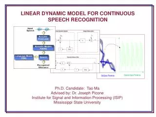
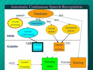
Statistical Speech Recognition • In this presentation, language model is assumed to be given in advance while acoustic model is needed to be estimated • HMMs (hidden Markov models) are widely adopted for acoustic modeling Speech Acoustic Match Linguistic Decoding Feature Extraction Recognized Sentence
Expected Risk • Let be a finite set of various possible word sequences for a given observation utterance • Assume that the true word sequence is also in • Let be the action of classifying a given observation sequence to a word sequence • Letbe the loss incurred when we take such an action (and the true word sequence is just ) • Therefore, the (expected) risk for a specific action [Duda et al. 2000]
Decoding: Minimum Expected Risk (1/2) • In speech recognition, we can take the action with the minimum (expected) risk • If zero-one loss function is adopted (string-level error) • Then
Decoding: Minimum Expected Risk (2/2) • Thus, • Select the word sequence withmaximum posterior probability (MAP decoding) • The string editing or Levenshtein distance also can be accounted for the loss function • Take individual word errors into consideration • E.g., Minimum Bayes Risk (MBR) search/decoding [V. Goel et al. 2004], Word Error Minimization [Mangu et al. 2000]
Training: Minimum Overall Expected Risk (1/2) • In training, we should minimize the overall (expected) loss of the actions of the training utterances • is the true word sequence of • The integral extends over the whole observation sequence space • However, when a limited number of training observation sequences are available, the overall risk can be approximated by
Training: Minimum Overall Expected Risk (2/2) • Assume to be uniform • The overall risk can be further expressed as • If zero-one loss function is adopted • Then
Training: Minimum Error Rate • Minimum Error Rate (MER) estimation • MER is equivalent to MAP
Training: Maximum Likelihood (1/2) • The objective function of Maximum Likelihood (ML) estimation can be obtained if Jensen Inequality is further applied • Maximize the overall log-posterior of all training utterances minimize the upper bound [Schlüter 2000] Independent of uniform
Training: Maximum Likelihood (2/2) • On the other hand, the discriminative training approaches attempt to optimize the correctness of the model set by formulating an objective function that in some way penalizes the model parameters that are liable to confuse correct and incorrect answers • MLE can be considered as a derivation from overall log-posterior
Training: Maximum Mutual Information (1/3) • The objective function can be defined as the sum of the pointwise mutual information of all training utterances and their associated true word sequences • The maximum mutual information (MMI) estimation tries to find a new parameter set ( ) that maximizes the above objective function [Bahl et al. 1986]
Training: Maximum Mutual Information (2/3) • An alternative derivation based on the overall expected risk criterion • Which is equivalent to the maximization of overall log-posterior of all training utterances Independent of include
Training: Maximum Mutual Information (3/3) • When we maximize the MMIE objection function • Not only the probability of true word sequence (numerator, like the MLE objective function) can be increased, but also can the probabilities of other possible word sequences (denominator) be decreased • Thus, MMIE attempts to make the correct hypothesis more probable, while at the same time it also attempts to make incorrect hypotheses less probable • MMIE also can be considered as a derivation from overall log-posterior
Training: Minimum Classification Error (1/2) • The misclassification measure is defined as • Minimization of the overall misclassification measure is similar to MMIE when language model is assumed uniformly distributed [Chou 2000]
Training: Minimum Classification Error (2/2) • Embed a sigmoid (loss) function to smooth the misclassification measure • Let and , then we have • Minimization of the overall loss directly minimizes (classification) error rate, so MCE can be regarded as a derivation from MER
Training: Minimum Phone Error • The objective function of Minimum Phone Error (MPE) is directly derived from the overall expected risk criterion • Replace the loss function with the so-called accuracy function • MPE tries to maximize the expected (phone or word) accuracy of all possible word sequences (generated by the recognizer) regarding the training utterances [Povey 2004]
Objective Function Optimization • Objective function has the “latent variable” problem, such that it can not be directly optimized Iterative optimization • Gradient-based approaches • E.g., MCE • Expectation Maximum (EM) • strong-sense auxiliary function • E.g., MLE • Weak-sense auxiliary function • E.g., MMIE, MPE
Three Steps for EM • Step 1.Draw a lower bound • Use the Jensen’s inequality • Step 2.Find the best lower bound auxiliary function • Let the lower bound touch the objective function at current guess • Step 3.Maximize the auxiliary function • Obtain the new guess • Go to Step 2 until converge [Minka 1998]
Step 1.Draw a lower bound (1/3) objective function current guess
Step 1.Draw a lower bound (2/3) objective function lower bound function
Step 1.Draw a lower bound (3/3) Apply Jensen’s Inequality The lower bound function of
Step 2.Find the best lower bound (1/4) objective function lower bound function
Step 2.Find the best lower bound (2/4) • Let the lower bound touch the objective function at current guess • Find the best at
After derivation w.r.t Step 2.Find the best lower bound (3/4) Set it to zero
Step 2.Find the best lower bound (4/4) Q function
Step 3.Maximize the auxiliary function (1/3) auxiliary function
Step 3.Maximize the auxiliary function (2/3) objective function
Step 3.Maximize the auxiliary function (3/3) objective function
Step 2.Find the best lower bound objective function auxiliary function
Step 3.Maximize the auxiliary function objective function
Strong-sense Auxiliary Function • If is said to be a strong-sense auxiliary function for around ,iff [Povey et al. 2003]
Weak-sense Auxiliary Function (1/5) • If is said to be a weak-sense auxiliary function for around ,iff
Weak-sense Auxiliary Function (2/5) objective function auxiliary function
Weak-sense Auxiliary Function (3/5) objective function auxiliary function
Weak-sense Auxiliary Function (4/5) objective function
Weak-sense Auxiliary Function (5/5) • If is said to be a smooth function around ,iff • Speed up convergence • Provide more stable estimate
Smooth Function (1/2) objective function smooth function
Smooth Function (2/2) objective function is also a weak-sense auxiliary function
MPE: Discrimination • The MPE objective function is less sensitive to portions of the training data that are poorly transcribed • A (word) lattice structure can be used here to approximate the set of all possible word sequences of each training utterance • Training statistics can be efficiently computed via such structure
MPE: Auxiliary Function (1/2) • The weak-sense auxiliary function for MPE model updating can be defined as • is a scalar value (a constant) calculated for each phone arc q, and can be either positive or negative (because of the accuracy function) • The auxiliary function also can be decomposed as still have the “latent variable” problem arcs with positive contributions (so-called numerator) arcs with negative contributions (so-called denominator)
MPE: Auxiliary Function (2/2) • The auxiliary function can be modified by considering the normal auxiliary function for • The smoothing term is not added yet here • The key quantity (statistics value) required in MPE training is , which can be termed as
MPE: Statistics Accumulation (1/2) • The objective function can be expressed as (for a specific phone arc ) • The differential can be expressed as
MPE: Statistics Accumulation (2/2) The average accuracy of sentences passing through the arc q The likelihood of the arc q The average accuracy of all the sentences in the word graph
MPE: Accuracy Function (1/4) • and can be calculated in an approximation way using the word graph and the Forward-Backward algorithm • Note that the exact accuracy function is express as the sum of phone-level accuracy over all phones , e.g. • However, such accuracy is obtained by full alignment between the true and all possible word sequences, which is computational expensive
MPE: Accuracy Function (2/4) • An approximated phone accuracy is defined • : the ration of the portion of that is overlapped by 1. Assume the true word sequence has no pronunciation variation 2. Phone accuracy can be obtained by simple local search 3. Context-independent phones can be used for accuracy calculation
Forward for 開始時間為0的音素q end for t=1 to T-1 for 開始時間為t的音素q for 結束時間為t-1且可連至q的音素r end for 結束時間為t-1且可連至q的音素r end endend MPE: Accuracy Function (3/4) • Forward-Backward algorithm for statistics calculation • Use “phone graph” as the vehicle
MPE: Accuracy Function (4/4) for 結束時間為T-1的音素q for t=T-2 to 0 for 結束時間為t的音素q for 開始時間為t+1且可連至q的音素r end for 開始時間為t+1且可連至q的音素r end end end Backward for 每一音素q end
MPE: Smoothing Function • The smoothing function can be defined as • The old model parameters( ) are used here as the hyper-parameters • It has a maximum value at
MPE: Final Auxiliary Function (1/2) weak-senseauxiliary function strong-sense auxiliary function smoothing function involved weak-sense auxiliary function
Weak-sense auxiliary function Strong-senseauxiliary Weak-sense Add smooth function MPE: Final Auxiliary Function (2/2)