NONLINEAR DYNAMIC INVARIANTS FOR CONTINUOUS SPEECH RECOGNITION

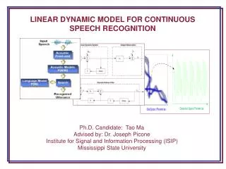
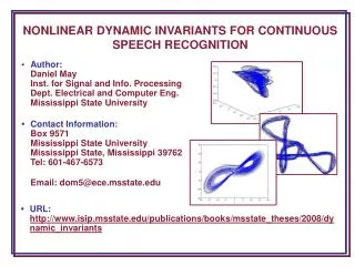
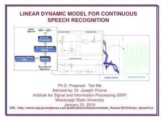
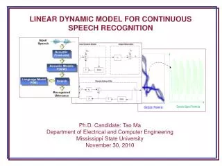
1. NONLINEAR DYNAMIC INVARIANTS FOR CONTINUOUS SPEECH RECOGNITION • Author: Daniel May Mississippi State University • Contact Information: 1255 Louisville St. Apt 7 Starkville, MS 39759 Tel: 601-467-6573 Email: MSUdom5@gmail.com • URL: http://www.isip.msstate.edu/publications/books/msstate_theses/2008/dynamic_invariants

2. Abstract In this work, nonlinear acoustic information is combined with traditional linear acoustic information in order to produce a noise-robust set of features for speech recognition. Classical acoustic modeling techniques for speech recognition have relied on a standard assumption of linear acoustics where signal processing is primarily performed in the signal's frequency domain. While these conventional techniques have demonstrated good performance under controlled conditions, the performance of these systems suffers significant degradations when the acoustic data is contaminated with previously unseen noise. The objective of this thesis was to determine whether nonlinear dynamic invariants are able to boost speech recognition performance when combined with traditional acoustic features. Several sets of experiments are used to evaluate both clean and noisy speech data. The invariants resulted in a maximum relative increase of 11.1% for the clean evaluation set. However, an average relative decrease of 7.6% was observed for the noise-contaminated evaluation sets. The fact that recognition performance decreased with the use of dynamic invariants suggests that additional research is required for robust filtering of phase spaces constructed from noisy time-series.

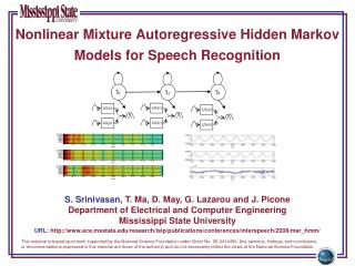
3. Motivation • Traditional MFCCs features capture the lower-order characteristics of the speech production process. • Experimental evidence [Teager and Teager] has suggested the existence of nonlinear mechanisms in the production of speech. • Nonlinear dynamic invariants can describe these mechanisms and are able to discriminate between different types of speech. • Dynamic invariants capture the higher-order information missed by traditional linear features. • Research [Pitsikalis and Maragos] has suggested that dynamic invariants are robust to previously unseen recording conditions. • Combining dynamic invariants with MFCCs should produce a more robust feature vector for continuous speech recognition.

4. Traditional Features for Speech • Traditional Linear Features • Based on the source-filter model • Model the vocal tract as a linear filter • Features are extracted from the frequency domain of the signal • Mel-Frequency Cepstral Coefficients • 10 ms frame duration • 25 ms Hamming window • Absolute energy • 12 cepstral coefficients • First and second derivatives Input Speech Zero-mean and Pre-emphasis Fourier Transf. Analysis Energy Cepstral Analysis Δ / ΔΔ

5. Nonlinear Invariant Features for Speech Input Speech • Dynamic Systems • Defined by a set of first-order ordinary differential equations. • Phase space describes the behavior of the system's dynamic variables as time evolves • Time evolution of the system forms a path, or trajectory within the phase space • The system’s attractor is the subset of the phase space to which the trajectory settles after a long period of time • Nonlinear Invariant Features • Computed from the time domain signal • Signal is an observable of a dynamic systems • Phase space is reconstructed from observable • Invariants estimated based on properties of the phase space Zero-mean Phase Space Reconstruction Dynamic Invariant Estimation

6. Phase Space Reconstruction (RPS) • Time Delay Embedding • Simplest reconstruction method • Reconstructs phase space using time-delayed copies of the original time series. • Correct choices for time delay τ and embedding dimensions m are important • SVD Embedding • More robust to noise than time-delay embedding • SVD is applied to a time-delay RPS to smooth trajectories • Example: Lorenz System Observed x Variable Reconstructed Phase Space (RPS) Original Lorenz System

7. Lyapunov Exponents • Measures the level of chaos in the reconstructed attractor • Computed by analyzing the relative behavior of neighboring trajectories within the attractor • Example: • Final Lyapunov exponent is the average trajectory behavior over the entire attractor Stable Trajectories (~0) Converging Trajectories (<0) Diverging Trajectories (>0)

8. Lyapunov Exponents Examples • Reconstructed attractor for phoneme /m/ • On average, neighboring trajectories remain close together as time evolves • This behavior results in a relatively low exponent (λ=-8.96) • Reconstructed attractor for phoneme /f/ • Neighboring trajectories diverge quickly as time evolves • This behavior results in a relatively high exponent (λ=566.11)

9. Fractal Dimension • Quantifies the geometrical complexity of the attractor by measuring self-similarity • Self-similarity example: Sierpinski Triangle • Computed by estimating the attractor’s correlation integral which measures the extent to which the attractor fills the phase space • The method for finding fractal dimension from a time-series is called correlation dimension, and is found from the correlation integral using:

10. Fractal Dimension Examples • Reconstructed attractor for phoneme /aa/. • Self similarity clearly visible in the symmetric shape of the attractor. • This attractor results in a correlation dimension of 0.88. • Reconstructed attractor for phoneme /eh/. • Self-similarity not as obvious, but can be seen in the ‘jagged’ structures of the attractor. • This attractor results in a correlation dimension of 0.61.

11. Kolmogorov Entropy • Measures the average rate of information production of a dynamic system • Like Fractal Dimension, Kolmogorov entropy (K2) is related to the correlation integral of the attractor: • The method used to estimate entropy is called correlation entropy and is defined by: • Examples: Phoneme /aa/ = 666.0 Phoneme /f/ = 964.6 Phoneme /m/ = 343.4

12. Measuring Dynamic Invariants of Speech Signals • Dynamic invariants are estimated from segments of the speech signal • These segments are aligned with the signal frames from which MFCCs are computed • The length of the signal segment varies depending on which invariant is being estimated

13. Experimentation Strategy • Use the WSJ-derived Aurora corpus for evaluations • Perform a set of low-level phonetic classification experiments to better understand the effects of adding dynamic invariants to MFCC features • Establish standard MFCC baseline performance • Evaluate noise-free Aurora test set using MFCC/dynamic invariant combinations • Evaluate mismatched Aurora test conditions using MFCC/dynamic invariant combinations

14. Aurora Corpus Description • Acoustic Training: • Derived from 5000 word WSJ0 task • 16 kHz sample rate • Recorded with Sennheiser microphone • 83 speakers • 7138 training utterances totaling in 14 hours of speech • Development Sets: • Derived from WSJ0 Evaluation and Development sets • 7 individual test sets recorded with Sennheiser microphone • Clean set plus 6 sets with noise conditions • Randomly chosen SNR between 5 and 15 dB for noisy sets

15. Pilot Experiments • Phonetic classification experiments are used to assess the extent to which dynamic invariants are able to represent speech • Each dynamic invariant is combined with the MFCC features to produce three new feature vectors. • Using time-alignments of the training data, a 16-mixture GMM is trained for each of the 40 phonemes present in the data • Signal frames of the training data are then each classified as one of the phonemes. • Each new feature vector resulted in an overall classification increase. • The results suggest that improvements can be expected for larger scale speech recognition experiments

16. Continuous Speech Recognition Experiments • Baseline System • Adapted from previous Aurora Evaluation Experiments • Uses 39 dimension MFCC features • Uses state-tied 4-mixture cross-word triphone acoustic models • Model parameters estimated using Baum-Welch algorithm • Viterbi beam search used for evaluations • Four different feature combinations were used for these evaluations and compared to the baseline: • The statistical significance of the results for each experiment are also computed

17. Results for Clean Evaluation Sets • Each of the four feature sets resulted in a recognition accuracy increase for the clean evaluation set. • Results with a significance level of 0.001 (0.1%) are considered to be statistically significant. • Although each feature set saw a WER decrease, the improvement for FS3 was the only one found to be statistically significant with a relative improvement of 11% over the baseline system.

18. Results for Noisy Evaluation Sets • Most of the noisy evaluation sets resulted in a recognition accuracy decrease. • FS3 resulted in a slight improvement for a few of the evaluation sets, but these improvements are not statistically significant • The average relative performance decrease was around 7% for FS1 and FS2 and around 14% for FS4. • The performance degradations seem to contradict the theory that dynamic invariants are noise-robust.

19. Computational Issues • Extracting features from a phase space is computationally expensive. • Computation methods require traversing the phase space many times and making computations for each state. • Advanced phase space filtering methods increase computational costs significantly. • Parallelizing the algorithm could cut computational costs. • Further research should investigate and develop optimized algorithms for phase-space related computations.

20. Conclusions • The recognition performance improvements for the noise-free data suggest that nonlinear dynamic invariants can be combined with MFCCs to better model speech. • The use of correlation entropy resulted in the most significant performance increase with a relative improvement of 11% over the baseline. • Dynamic invariants did not improve the recognition results for the noisy evaluation sets, and in most cases, resulted in a performance decrease. • The use of correlation entropy resulted in a slight WER decrease for some of the noisy sets, but these were not significant. • It is likely that frame-based feature extraction method does not provide the algorithms with enough data to accurately estimate the invariants. • For noisy time series, more data is needed to accurately capture the dynamics of the reconstructed attractor.

21. Future Work • While SVD embedding has been shown to reduce the effects of noise, it is not very effective for speech since the time-series used for phase space reconstruction is limited by the short frame length. Therefore, more research is required for the development of advanced phase space filtering techniques which can be used to post-process a reconstructed phase space and reduce the effects of noise on phase space dynamics. • Instead of computing values which describe the global behavior of the attractor, such as dynamic invariants, it may be beneficial to model the attractor itself. This would require a new type of statistical model and would provide a more complete description of the local dynamics within the attractor.

22. Other Related Interests • Advanced Acoustic Modeling Techniques • Spoken Term Detection • Speaker Recognition • Hardware Acceleration of Speech Recognition Applications (See LLNL Work) • Graphics and GPU Programming

23. Brief Bibliography • A. Kumar and S. K. Mullick, “Nonlinear Dynamical Analysis of Speech,” Journal of the Acoustical Society of America, vol. 100, no. 1, pp. 615-629, July 1996. • H. M. Teager and S. M. Teager, “Evidence for Nonlinear Production Mechanisms in the Vocal Tract,” NATO Advanced Study Institute on Speech Production and Speech Modeling, Bonas, France, pp. 241-261, July 1989. • V. Pitsikalis and P. Maragos, “Filtered Dynamics and Fractal Dimensions for Noisy Speech Recognition,” IEEE Signal Processing Letters, vol. 13, no. 11, pp. 711-714, November 2006. • M. Banbrook, G. Ushaw, and S. McLaughland, “How to Extract Lyapunov Exponents from Short and Noisy Time Series,” IEEE Transactions on Signal Processing, vol. 45, no. 5, pp. 1378-1382, May 1997. • P. Grassberger and I. Procaccia, “Estimation of the Kolmogorov Entropy from a Chaotic Signal,” Physical Review A, vol. 28, no. 4, pp. 2591-2594, October 1983. • H. F. V. Boshoff and M. Grotepass, “The Fractal Dimension of Fricative Speech Sounds,” Proceedings of the South African Symposium on Communication and Signal Processing, pp. 12-16, Pretoria, South Africa, August 1991.

24. Aurora Project Website: recognition toolkit, multi-CPU scripts, database definitions, publications, and performance summary of the baseline MFCC front end • Speech Recognition Toolkits: compare front ends to standard approaches using a state of the art ASR toolkit Available Resources

25. Related Coursework