Download
1 / 44
440 likes | 475 Views
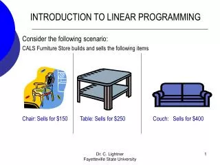
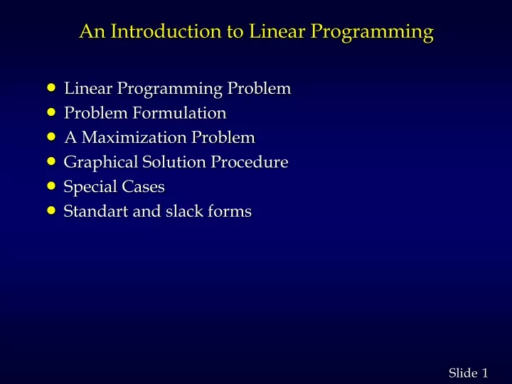
An Introduction to Linear Programming. Linear Programming Problem Problem Formulation A Maximization Problem Graphical Solution Procedure Special Cases Standart and slack forms. Linear Programming (LP) Problem.

E N D
An Introduction to Linear Programming • Linear Programming Problem • Problem Formulation • A Maximization Problem • Graphical Solution Procedure • Special Cases • Standart andslackforms
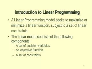
Linear Programming (LP) Problem • A mathematical programming problem is one that seeks to maximize an objective function subject to constraints. • If both the objective function and the constraints are linear, the problem is referred to as a linear programming problem. • Linear functions are functions in which each variable appears in a separate term raised to the first power and is multiplied by a constant (which could be 0). • Linear constraints are linear functions that are restricted to be "less than or equal to", "equal to", or "greater than or equal to" a constant.
LP Solutions • The maximization or minimization of some quantity is the objective in all linear programming problems. • A feasible solution satisfies all the problem's constraints. • An optimal solution is a feasible solution that results in the largest possible objective function value when maximizing (or smallest when minimizing). • A graphical solution method can be used to solve a linear program with two variables.
Problem Formulation • Problem formulation or modeling is the process of translating a verbal statement of a problem into a mathematical statement.
Guidelines for Model Formulation • Understand the problem thoroughly. • Write a verbal description of the objective. • Write a verbal description of each constraint. • Define the decision variables. • Write the objective in terms of the decision variables. • Write the constraints in terms of the decision variables.
Example Example Maximize: Z = 3 X1 + 5 X2 Subject to X1 <= 4 2X2 <=12 3X1 + 2X2 <=18 X1, X2 >=0
Example 1: A Maximization Problem • LP Formulation Max z = 5x1 + 7x2 s.t. x1< 6 2x1 + 3x2< 19 x1 + x2< 8 x1, x2> 0
Example 1: Graphical Solution • Constraint #1 Graphed x2 8 7 6 5 4 3 2 1 1 2 3 4 5 6 7 8 9 10 x1< 6 (6, 0) x1
Example 1: Graphical Solution • Constraint #2 Graphed x2 8 7 6 5 4 3 2 1 1 2 3 4 5 6 7 8 9 10 (0, 6 1/3) 2x1 + 3x2< 19 (9 1/2, 0) x1
Example 1: Graphical Solution • Constraint #3 Graphed x2 (0, 8) 8 7 6 5 4 3 2 1 1 2 3 4 5 6 7 8 9 10 x1 + x2< 8 (8, 0) x1
Example 1: Graphical Solution • Combined-Constraint Graph x2 x1 + x2< 8 8 7 6 5 4 3 2 1 1 2 3 4 5 6 7 8 9 10 x1< 6 2x1 + 3x2< 19 x1
Example 1: Graphical Solution • Feasible Solution Region x2 8 7 6 5 4 3 2 1 1 2 3 4 5 6 7 8 9 10 Feasible Region x1
Example 1: Graphical Solution • Objective Function Line x2 8 7 6 5 4 3 2 1 1 2 3 4 5 6 7 8 9 10 (0, 5) 5x1 + 7x2 = 35 (7, 0) x1
Example 1: Graphical Solution • Optimal Solution x2 8 7 6 5 4 3 2 1 1 2 3 4 5 6 7 8 9 10 5x1 + 7x2 = 46 Optimal Solution x1
Summary of the Graphical Solution Procedurefor Maximization Problems • Prepare a graph of the feasible solutions for each of the constraints. • Determine the feasible region that satisfies all the constraints simultaneously.. • Draw an objective function line. • Move parallel objective function lines toward larger objective function values without entirely leaving the feasible region. • Any feasible solution on the objective function line with the largest value is an optimal solution.
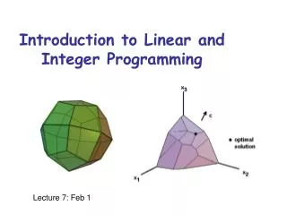
Extreme Points and the Optimal Solution • The corners or vertices of the feasible region are referred to as the extreme points. • An optimal solution to an LP problem can be found at an extreme point of the feasible region. • When looking for the optimal solution, you do not have to evaluate all feasible solution points. • You have to consider only the extreme points of the feasible region.
Example 1: Graphical Solution • The Five Extreme Points 8 7 6 5 4 3 2 1 1 2 3 4 5 6 7 8 9 10 5 4 Feasible Region 3 1 2 x1
Example 2: A Minimization Problem • LP Formulation Min z = 5x1 + 2x2 s.t. 2x1 + 5x2> 10 4x1 - x2> 12 x1 + x2> 4 x1, x2> 0
Example 2: Graphical Solution • Graph the Constraints Constraint 1: When x1 = 0, then x2 = 2; when x2 = 0, then x1 = 5. Connect (5,0) and (0,2). The ">" side is above this line. Constraint 2: When x2 = 0, then x1 = 3. But setting x1 to 0 will yield x2 = -12, which is not on the graph. Thus, to get a second point on this line, set x1 to any number larger than 3 and solve for x2: when x1 = 5, then x2 = 8. Connect (3,0) and (5,8). The ">" side is to the right. Constraint 3: When x1 = 0, then x2 = 4; when x2 = 0, then x1 = 4. Connect (4,0) and (0,4). The ">" side is above this line.
Example 2: Graphical Solution • Constraints Graphed x2 Feasible Region 5 4 3 2 1 4x1 - x2> 12 x1 + x2> 4 2x1 + 5x2> 10 1 2 3 4 5 6 x1
Example 2: Graphical Solution • Graph the Objective Function Set the objective function equal to an arbitrary constant (say 20) and graph it. For 5x1 + 2x2 = 20, when x1 = 0, then x2 = 10; when x2= 0, then x1 = 4. Connect (4,0) and (0,10). • Move the Objective Function Line Toward Optimality Move it in the direction which lowers its value (down), since we are minimizing, until it touches the last point of the feasible region, determined by the last two constraints.
Example 2: Graphical Solution • Objective Function Graphed Min z = 5x1 + 2x2 4x1 - x2> 12 x1 + x2> 4 x2 5 4 3 2 1 2x1 + 5x2> 10 1 2 3 4 5 6 x1
Example 2: Graphical Solution • Solve for the Extreme Point at the Intersection of the Two Binding Constraints 4x1 - x2 = 12 x1+ x2 = 4 Adding these two equations gives: 5x1 = 16 or x1 = 16/5. Substituting this into x1 + x2 = 4 gives: x2 = 4/5 • Solve for the Optimal Value of the Objective Function Solve for z = 5x1 + 2x2 = 5(16/5) + 2(4/5) = 88/5. Thus the optimal solution is x1 = 16/5; x2 = 4/5; z = 88/5
Example 2: Graphical Solution • Optimal Solution Min z = 5x1 + 2x2 4x1 - x2> 12 x1 + x2> 4 x2 5 4 3 2 1 2x1 + 5x2> 10 Optimal: x1 = 16/5 x2 = 4/5 1 2 3 4 5 6 x1
Special Cases • Alternative Optimal Solutions In the graphical method, if the objective function line is parallel to a boundary constraint in the direction of optimization, there are alternate optimal solutions, with all points on this line segment being optimal. • Infeasibility A linear program which is overconstrained so that no point satisfies all the constraints is said to be infeasible. • Unbounded (See example on upcoming slide.)
Example: Infeasible Problem • Solve graphically for the optimal solution: Max z = 2x1 + 6x2 s.t. 4x1 + 3x2< 12 2x1 + x2> 8 x1, x2> 0
Example: Infeasible Problem • There are no points that satisfy both constraints, hence this problem has no feasible region, and no optimal solution. x2 2x1 + x2> 8 8 4x1 + 3x2< 12 4 x1 3 4
Example: Unbounded Problem • Solve graphically for the optimal solution: Max z = 3x1 + 4x2 s.t. x1 + x2> 5 3x1 + x2> 8 x1, x2> 0
Example: Unbounded Problem • The feasible region is unbounded and the objective function line can be moved parallel to itself without bound so that z can be increased infinitely. x2 3x1 + x2> 8 8 Max 3x1 + 4x2 5 x1 + x2> 5 x1 2.67 5
Convertinglinearprogramsinto standart form • A linear program may not be in standart form forone of fourpossiblereasons: • Theobjectivefunctionmay be a minimizationratherthan a maximization • Theremay be variableswithoutnonnegativlyconstraints • Theremay be equalityconstraintswhichhave an equalsignratherthan a lessthan-orequal-tosign • Theremay be inequalityconstraints but instead of having a less-thantheyhave a greaterthanorequaltosign.
Converting to Standard Form • If variable xj doesn’t have a non-negativity constraint: • Replace each occurrence of xj (in constraints and objective function) by xj+-xj- • Add non-negativity constraints: xj+, xj- 0
Convertinginto standart form • Toconvert a mimimizationlinear program into an equivalentmaximizationlinear program wesimplynegatethecoefficients in theobjectivefunction • Forexample • Subjectto
Convertinginto standart form • Wenegatethecoefficients of theobjectivefunctionandweobtain
Convertinto standart form • Nowwereplace • Nowwehavethe problem
Convertinto standart form • Nextweconvertequalityconstraintsintoinequalityconstraints.
Convertinginto standart form • Finally, wenegate >= constraint. Forconsistency in variablenameswerenamevariables.
Convertinglinear program intoslack form • Let • be an inequalityconstraint. Weintroduce a newvariable s andrewriteinequality as twoconstraints
Convertingintoslack form • Wecall s a slackvariablebecause it measurestheslack, ordifferencebetweentheleft-handandright-handsides of equation. • Forexamplewe can rewriteour problem in slack form • Our problem in standart form is thefollowing:
Weindtroduceslackvariables Obtainingthe problem in slack form