INTRODUCTION TO LINEAR PROGRAMMING

1. INTRODUCTION TO LINEAR PROGRAMMING CONTENTS • Introduction to Linear Programming • Applications of Linear Programming Reference: Chapter 1 in BJS book.

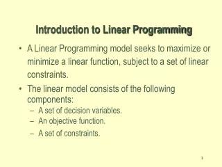
2. Linear Programming Problem • Features of Linear programming problem: • Decision Variables • We maximize (or minimize) a linear function of decision variables, called objective function. • The decision variables must satisfy a set of constraints. • Decision variables have sign restrictions. • Example: Maximize z = 3x1 + 2x2 subject to 2x1 + x2 100 x1 + x2 80 x1 40 x1, x2 0

3. A Typical Linear Programming Problem Linear Programming Formulation: Minimize c1x1 + c2x2 + c3x3 + …. + cnxn subject to a11x1 + a12x2 + a13x3 + …. + a1nxn  b1 a21x1 + a22x2 + a23x3 + …. + a2nxn  b2 : : am1x1 + am2x2 + am3x3 + …. + amnxn bm x1, x2, x3 , …., xn 0 or, Minimize j=1, n cjxj subject to j=1, n aijxj -xn+i = bi for all i = 1, …, m xj  0 for all j =1, …, n+m Linear Objective • Linear Constraints; • - Technology • Uncontrolable • variables/factors Decision (controlable) variables - Can take any real value - Restricted or unrestrited in sign Standard form representation

4. Matrix Notation Minimize cx subject to Ax = b x  0 where

5. Linear Programming Modeling and Examples • Stages of an application: • Problem formulation • Mathematical model • Deriving a solution • Model testing and analysis • Implementation

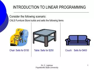
6. An Example of a LP • Giapetto’s woodcarving manufactures two types of wooden toys: soldiers and trains. How many of each type to produce? Constraints: • 100 finishing hour per week available • 80 carpentry hours per week available • produce no more than 40 soldiers per week • Objective: maximize profit? Minimize cost?

7. An Example of a LP (cont.) Linear Programming formulation: Maximize z = 3x1 + 2x2(Obj. Func.) subject to 2x1 + x2 100 (Finishing constraint) x1 + x2 80 (Carpentry constraint) x1 40 (Bound on soldiers) x1 0 (Sign restriction) x2 0 (Sign restriction)

8. Assumptions of Linear Programming • Proportionality Assumption • Contribution of a variable is proportional to its value. • Additivity Assumptions • Contributions of variables are independent. • Divisibility Assumption • Decision variables can take fractional values. • Certainty Assumption • Each parameter is known with certainty.

9. Capital Budgeting Problem • Five different investment opportunities are available for investment. • Fraction of investments can be bought. • Money available for investment: Time 0: $40 million Time 1: $20 million • Maximize the Net Present Value of all investments.

10. Transportation Problem • The Brazilian coffee company processes coffee beans into coffee at m plants. The production capacity at plant i is ai. • The coffee is shipped every week to n warehouses in major cities for retail, distribution, and exporting. The demand at warehouse j is bj. • The unit shipping cost from plant i to warehouse j is cij. • It is desired to find the production-shipping pattern xij from plant i to warehouse j, i = 1, .. , m, j = 1, …, n, that minimizes the overall shipping cost. • What is Xij? Produced? Shipped? • Why not consider production and shipping together? • Why not maximize profit?

11. Static Workforce Scheduling • Number of full time employees on different days of the week are given below. • Each employee must work five consecutive days and then receive two days off. • The schedule must meet the requirements by minimizing the total number of full time employees. • Decision variable?

12. Multi-Period Financial Models • Determine investment strategy for the next three years • Money available for investment at time 0 = $100,000 • Investment opportunities available : A, B, C, D & E • No more than $75,000 in one invest • Uninvested cash earns 8% interest • Cash flow of these investments: • Decision variables?

13. Cutting Stock Problem • A manufacturer of metal sheets produces rolls of standard fixed width w and of standard length l. • A large order is placed by a customer who needs sheets of width w and varying lengths. He needs bi sheets of length li, i = 1, …, m. • The manufacturer would like to cut standard rolls in such a way as to satisfy the order and to minimize the waste. • Since scrap pieces are useless to the manufacturer, the objective is to minimize the number of rolls needed to satisfy the order.

14. Multi-Period Workforce Scheduling • Requirement of skilled repair time (in hours) is given below. • At the beginning of the period, 50 skilled technicians are available. • Each technician is paid $2,000 and works up to 160 hrs per month. • Each month 5% of the technicians leave. • A new technician needs one month of training, is paid $1,000 per month, and requires 50 hours of supervision of a trained technician. • Meet the service requirement at minimum cost.

15. Solution: Capital Budgeting Problem Decision Variables: xi: fraction of investment i purchased Formulation: Maximize z = 17x1 + 16x2 + 16x3 + 14x4 + 39x5 subject to 11x1 + 53x2 + 5x3 + 5x4 + 29x5 £ 40 3x1 + 6x2 + 5x3 + x4 + 34x5 £ 20 x1£ 1 x2£ 1 x3£ 1 x4£ 1 x5£ 1 x1, x2, x3, x4, x5³ 0

16. Solution: Transportation Problem Decision Variables: xij: amount shipped from plant i to warehouse j Formulation: Minimize z = subject to = ai, i = 1, … , m  bj, j = 1, … , n xij 0, i = 1, … , m, j = 1, … , n

17. Solution: Static Workforce Scheduling LP Formulation: Min. z = x1+ x2 + x3 + x4 + x5 + x6 + x7 subject to x1 + x4 + x5 + x6 + x7³17 x1+ x2 + x5 + x6 + x7³13 x1+ x2 + x3 + x6 + x7 ³15 x1+ x2 + x3 + x4 + x7³19 x1+ x2 + x3 + x4 + x5³14 x2 + x3 + x4 + x5 + x6³16 x3 + x4 + x5 + x6 + x7³11 x1, x2, x3, x4, x5, x6, x7³ 0

18. Solution: Multi period Financial Model Decision Variables: A, B, C, D, E : Dollars invested in the investments A, B, C, D, and E St: Dollars invested in money market fund at time t (t = 0, 1, 2) Formulation: Maximize z = B+ 1.9D+ 1.5E+ 1.08S2 subject to A+ C+ D+ S0 = 100,000 0.5A+ 1.2C+ 1.08S0 = B + S1 A+ 0.5B+ 1.08S1 = E + S2 A £ 75,000 B £ 75,000 C £ 75,000 D £ 75,000 E £ 75,000 A, B, C, D, E, S0, S1, S2³ 0

19. Solution: Multiperiod Workforce Scheduling Decision Variables: xt: number of technicians trained in period t yt: number of experienced technicians in period t Formulation: Minimize z = 1000(x1 + x2 + x3 + x4 + x5) + 2000(y1 + y2 + y3 + y4 + y5) subject to 160y1 - 50 x1³ 6000 y1 = 50 160y2 - 50 x2³ 7000 0.95y1 + x1 = y2 160y3 - 50 x3³ 8000 0.95y2 + x2 = y3 160y4 - 50 x4³ 9500 0.95y3 + x3 = y4 160y5 - 50 x5³11000 0.95y4 + x4 = y5 xt, yt³ 0, t = 1, 2, 3, … , 5

20. Cutting Stock Problem (contd.) • Given a standard sheet of length l, there are many ways of cutting it. Each such way is called a cutting pattern. • The jth cutting pattern is characterized by the column vector aj, where the ith component, namely, aij, is a nonnegative integer denoting the number of sheets of length li in the jth pattern. • Note that the vector aj represents a cutting pattern if and only if i=1,n aijli  l and each aij is a nonnegative number.

21. Cutting Stock Problem (contd.) Formulation: xi: Number of sheets cut using patter j Minimize i=1,n xi subject to i=1,n aij xi  bi i = 1, …, m xi  0 j = 1, …, n xi integer j = 1, …, n

22. Cutting Stock Problem (contd.) Formulation: Let l = 7, and type 1, type 2 and type 3 sizes demanded are 2, 3, and 5 with b1=10, b2=4, b4=3. possible patterns: j 3 2 0 1 i 0 1 2 0 0 0 0 1 Min. z = x1+ x2 + x3 + x4 subject to 3x1+2 x2 + x4 10 x2 + 2x3 4 x4 3 xj integer j = 1, …, 4

23. Modeling issues • Mini- max objective (scenario based modeling): => Minimizing the maximum regret in decision making under uncertain outcomes fi(x) is the cost of the outcome under scenario i (equally likely scenarios) fi(x)=return of best decision under scenario i – return of the decision as a solution of the model above

24. Modeling issues • Max-Min objective: =>

25. Modeling issues • Mini-max: • Example: Farmer problem; • How to allocate land to different crops? • There are 6 weather scenarios (cold, dry) (cold, rainy) (hot, dry) (hot, rainy) (warm, dry) (warm, rainy) • Three different crops with different per m2 harvest values under different scenarios. Different per kilo market value for each crop. • For each fixed scenario, there is an optimal allocation • What is the optimal solution for a given scenario? • Criterion: Minimize the maximum revenue lost (regret) • Maxi-min • Example: Farmer problem: • Criterion: Maximize the minimum revenue to be obtained • fi(x): Revenue obtained for a given solution under scenario i • Which one is the right model?

26. Modeling issues • Minimize/Maximize absolute value => For maximimization problems multiply objective with -1 and turn them into minimization problem

27. Modeling issues

28. Modeling issues • Is the absolute value a linear function? • A function is a linear function if it satisfies the following two conditons; • f(a+b)=f(a)+f(b) • f(ax)= af(x) (for any real “a” value) • For the absolute function, we can find a counter example easily; • Let f(x)=|x| • f(-1+3) = |-1+3|=2 but f(-1)+f(3) = 1+3 = 4 first condition is violated. Therefore absolute value is not a linear function (proof by contradiction)

29. Modeling issues • Fixed charge problem: Cost function with a fixed part

30. Modeling issues • Either-or constraints: • 1 out of k type constraints

31. Modeling issues • If-then constraints

32. Modeling issues • Piecewise linear functions f(x) b3 b4 b1 b2 x x= z(i)*bi+z(i+1)*b(i+1) where z(i)+z(i+1) = 1 i=0..3 f(x) = z(i)*f(bi)+z(i+1)*f(b(i+1)) where z(i)+z(i+1) = 1 i=0..3 Let y(i) = 1 if b(i) <= x <= b(i+1) y(i) = 0otherwise 4 binary variables and 4+1 convex-combination variables (z).

33. Modeling issues Piecewise linear functions

34. Modeling issues Piecewise linear functions; Alternative formulation This model is not correct

35. Examples for some modelling constructs • Consider the transportation model • Either or; Either we transfer from facility 3 to 4 or from 3 to 5, not both simultaneously. • If then; If we transfer from facility 3 to 4, we must not transfer from facility 3 to 5 (If X34>0 then X35<=0 (-X35>=0))

36. Geometric Solution • Steps of the geometric solution • Determine and draw the feasible region • Draw the c vector • Draw the iso cost lines (perpendicular to c vector) • Find the last point(s) that iso-cost lines touch the feasible region, when we move towards direction of –c (in minimization). This point (or points) is the optimal solution.

37. Geometric Solution 4. Find the optimal point(s) 3. Draw the iso-cost lines • Draw the feasible • region 2. Draw vector c minimization; move towards –c maximization move towards c as long as (x1,x2) is in feasible region

38. Geometric Solution

39. Unique finite optimal solution

40. Alternative finite optimal solution

41. Unbounded optimal solution It is always the case that a corner point is among the optimal solution, if there is a finite optimal solution.

42. Empty feasible region