Download
1 / 44
540 likes | 1.09k Views
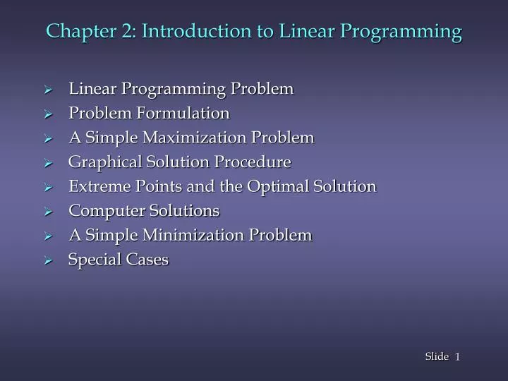
Chapter 2: Introduction to Linear Programming. Linear Programming Problem Problem Formulation A Simple Maximization Problem Graphical Solution Procedure Extreme Points and the Optimal Solution Computer Solutions A Simple Minimization Problem Special Cases. Linear Programming (LP) Problem.

E N D
Chapter 2: Introduction to Linear Programming • Linear Programming Problem • Problem Formulation • A Simple Maximization Problem • Graphical Solution Procedure • Extreme Points and the Optimal Solution • Computer Solutions • A Simple Minimization Problem • Special Cases
Linear Programming (LP) Problem • Linear programming (LP) involves choosing a course of action when the mathematical model of the problem contains only linear functions. (Note: Linear programming has nothing to do with computer programming.) • The maximization or minimization of some quantity is the objective in all linear programming problems. • All LP problems have constraints that limit the degree to which the objective can be pursued.
Linear Programming (LP) Terms • If both the objective function and the constraints are linear, the problem is referred to as a linear programming problem. • Linear functions are functions in which each variable appears in a separate term raised to the first power and is multiplied by a constant (which could be 0). • Linear constraints are linear functions that are restricted to be "less than or equal to", "equal to", or "greater than or equal to" a constant. • A feasible solution satisfies all the problem's constraints. • An optimal solution is a feasible solution that results in the largest possible objective function value when maximizing (or smallest when minimizing). • A graphical solution method can be used to solve a linear program with two variables.
Guidelines for Model Formulation Problem formulation or modeling is the process of translating a verbal statement of a problem into a mathematical statement. • Understand the problem thoroughly. • Describe the objective. • Describe each constraint. • Define the decision variables. • Write the objective in terms of the decision variables. • Write the constraints in terms of the decision variables. Note: Formulating models is an art that can only be mastered with practice and experience. Every LP problems has some unique features, but most problems also have common features.
LP Formulation: XYZ, Inc. XYZ, Inc. manufactures two products, namely Product 1 and Product 2. The profits for Products 1 and 2 are $5 and $7 per unit, respectively. Due to demand limitations XYZ, Inc. should not produce more than 6 units of Product 1. Both products are made from steel and wood. Product 1 needs 2 pounds of steel and 1 cubic foot of wood, while Product 2 needs to 3 pounds of steel and 1 cubic foot of wood. Currently XYZ, inc. has 19 pounds of steel and 8 cubic feet of wood. Formulate the problem above and determine the optimal solution. Describe the objective. Describe each constraint. Define the decision variables.
Example: XYZ, Inc. Mathematical Model Define the decision variables x1= number of units ofProduct 1 to produce x2= number of units ofProduct 2 to produce Objective: Maximize profit Maximize: 5x1 + 7x2 Constraint 1: Demand limitation of product 1 x1<6
Example: XYZ, Inc. (Continued) Mathematical Model Constraint 2: Steel Limitation 2x1 + 3x2 <19 Constraint 3: Wood Limitation x1 + x2 <8 Cannot produce negative units of products 1 and 2 x1> 0 and x2 >0.
XYZ, Inc.: A Simple Maximization Problem LP Formulation Objective Function Max 5x1 + 7x2 s.t. x1< 6 2x1 + 3x2< 19 x1 + x2< 8 x1> 0 and x2> 0 “Regular” Constraints Non-negativity Constraints
Example 1: Graphical Solution First Constraint Graphed x2 8 7 6 5 4 3 2 1 x1 = 6 (1: Product 1 Demand) Shaded region contains all feasible points for this constraint (6, 0) x1 1 2 3 4 5 6 7 8 9 10
Example 1: Graphical Solution • Second Constraint Graphed x2 8 7 6 5 4 3 2 1 (0, 61/3) 2x1 + 3x2 = 19 (2: Steel) Shaded region contains all feasible points for this constraint (91/2, 0) x1 1 2 3 4 5 6 7 8 9 10
Example 1: Graphical Solution • Third Constraint Graphed x2 (0, 8) 8 7 6 5 4 3 2 1 x1 + x2 = 8 (3: Wood) Shaded region contains all feasible points for this constraint (8, 0) x1 1 2 3 4 5 6 7 8 9 10
Example 1: Graphical Solution • Feasible region: collection of points that satisfy ALL constraints x2 x1 + x2 = 8 (3: Wood) 8 7 6 5 4 3 2 1 x1 = 6 (1: Demand) 2x1 + 3x2 = 19 (2: Steel) Feasible Region x1 1 2 3 4 5 6 7 8 9 10
Example 1: Graphical Solution • Objective Function Line x2 8 7 6 5 4 3 2 1 (0, 5) Objective Function 5x1 + 7x2 = 35 (7, 0) x1 1 2 3 4 5 6 7 8 9 10
Example 1: Graphical Solution • Selected Objective Function Lines x2 8 7 6 5 4 3 2 1 5x1 + 7x2 = 35 5x1 + 7x2 = 39 5x1 + 7x2 = 42 x1 1 2 3 4 5 6 7 8 9 10
Example 1: Graphical Solution • Optimal Solution x2 x2 x1 + x2= 8 (3: Wood) 8 7 6 5 4 3 2 1 8 7 6 5 4 3 2 1 Maximum Objective Function Line 5x1 + 7x2 = 46 Optimal Solution (x1 = 5, x2 = 3) x1 = 6 (1: Demand) Feasible Region 2x1 + 3x2 = 19 (2: Steel) x1 x1 1 2 3 4 5 6 7 8 9 10 1 2 3 4 5 6 7 8 9 10
Binding and Non-Binding Constraints • A Constraint is binding if its resource is completely usedup(i.e., no slack). Steel and wood constraints are binding. • Optimal Solution: (x1 = 5, x2 = 3) 2x1 + 3x2< 19 (2: Steel) x1 + x2< 8 (3: Wood) 2(5) + 3(3) = 19 5+3 = 8 • A constraint is not binding is its resource is not completely used up. Product 1 demand is not binding. x1< 6 (1: Demand) x1 = 5 (One unit left over called a ‘slack’)
Summary of the Graphical Solution Procedurefor Maximization Problems • Prepare a graph of the feasible solutions for each of the constraints. • Determine the feasible region that satisfies all the constraints simultaneously. • Draw an objective function line. • Move parallel objective function lines toward larger objective function values without entirely leaving the feasible region. • Any feasible solution on the objective function line with the largest value is an optimal solution.
Slack and Surplus Variables • A linear program in which all the variables are non-negative and all the constraints are equalities is said to be in standard form. • Standard form is attained by adding slack variables to "less than or equal to" constraints, and by subtracting surplus variables from "greater than or equal to" constraints. • Slack and surplus variables represent the difference between the left and right sides of the constraints. • Slack and surplus variables have objective function coefficients equal to 0.
Slack Variables (for < constraints) • Example 1 in Standard Form Max 5x1 + 7x2 + 0s1 + 0s2 + 0s3 s.t. x1 + s1 = 6 2x1 + 3x2 + s2 = 19 x1 + x2 + s3 = 8 x1, x2 , s1 , s2 , s3> 0 s1 , s2 , and s3 are slack variables
Slack Variables • Optimal Solution x2 Third Constraint: x1 + x2 = 8 First Constraint: x1 = 6 8 7 6 5 4 3 2 1 s3 = 0 s1 = 1 Second Constraint: 2x1 + 3x2 = 19 Optimal Solution (x1 = 5, x2 = 3) s2 = 0 x1 1 2 3 4 5 6 7 8 9 10
Extreme Points and the Optimal Solution • The corners or vertices of the feasible region are referred to as the extreme points. • An optimal solution to an LP problem can be found at an extreme point of the feasible region. • When looking for the optimal solution, you do not have to evaluate all feasible solution points. • You have to consider only the extreme points of the feasible region.
Example 1: Extreme Points x2 8 7 6 5 4 3 2 1 (0, 6 1/3) 5 (5, 3) 4 Feasible Region (6, 2) 3 (6, 0) (0, 0) 2 1 x1 1 2 3 4 5 6 7 8 9 10
Interpretation of Computer Output • LP problems involving 1000s of variables and 1000s of constraints are now routinely solved with computer packages. Linear programming solvers are now part of many spreadsheet packages, such as Microsoft Excel. • In this chapter we will discuss the following output: • objective function value • values of the decision variables • slack and surplus • In the next chapter we will discuss how an optimal solution is affected by a change in: • a coefficient of the objective function • the right-hand side value of a constraint • reduced costs
Computer Solutions: XYZ. Inc. • For MAN 321, we will use QM for Windows • Spreadsheet Showing Problem Data
Computer Solutions: XYZ. Inc. • Spreadsheet Showing Solution
Computer Solutions: XYZ. Inc. Spreadsheet Showing Ranging Note: Slacks/Surplus and Reduced Costs
Example 1: Spreadsheet Solution Interpretation of Computer Output We see from the Slides 24 and 25 that: Objective Function Value = 46 Decision Variable #1 (x1) = 5 Decision Variable #2 (x2) = 3 Slack in Constraint #1 = 6 – 5 = 1 Slack in Constraint #2 = 19 – 19 = 0 Slack in Constraint #3 = 8 – 8 = 0
Example 2: A Simple Minimization Problem LP Formulation Min 5x1 + 2x2 s.t. 2x1 + 5x2>10 (1) 4x1-x2>12 (2) x1 + x2>4 (3) x1, x2> 0
Example 2: Graphical Solution Graph the Constraints Constraint 1: When x1 = 0, then x2 = 2; when x2 = 0, then x1 = 5. Connect (5,0) and (0,2). The ">" side is above this line. Constraint 2: When x2 = 0, then x1 = 3. But setting x1 to 0 will yield x2 = -12, which is not on the graph. Thus, to get a second point on this line, set x1 to any number larger than 3 and solve for x2: when x1 = 5, then x2 = 8. Connect (3,0) and (5,8). The ">“ side is to the right. Constraint 3: When x1 = 0, then x2 = 4; when x2 = 0, then x1 = 4. Connect (4,0) and (0,4). The ">" side is above this line.
Example 2: Graphical Solution Constraints Graphed x2 6 5 4 3 2 1 Feasible Region 4x1-x2>12 (2) x1 + x2>4 (3) 2x1 + 5x2>10 (1) x1 1 2 3 45 6
Example 2: Graphical Solution Graph the Objective Function Set the objective function equal to an arbitrary constant (say 20) and graph it. For 5x1 + 2x2 = 20, when x1 = 0, then x2 = 10; when x2= 0, then x1 = 4. Connect (4,0) and (0,10). Move the Objective Function Line Toward Optimality Move it in the direction which lowers its value (down), since we are minimizing, until it touches the last point of the feasible region, determined by the last two constraints.
Example 2: Graphical Solution Objective Function Graphed x2 Min 5x1 + 2x2 6 5 4 3 2 1 4x1-x2>12 (2) x1 + x2>4 (3) 2x1 + 5x2>10 (1) x1 1 2 3 45 6
Example 2: Graphical Solution Solve for the Extreme Point at the Intersection of theTwo Binding Constraints 4x1 - x2 = 12 x1+ x2 = 4 Adding these two equations gives: 5x1 = 16 or x1 = 16/5 Substituting this into x1 + x2 = 4 gives: x2 = 4/5 Solve for the Optimal Value of the Objective Function 5x1 + 2x2 = 5(16/5) + 2(4/5) = 88/5
Example 2: Graphical Solution Optimal Solution x2 6 5 4 3 2 1 4x1-x2>12 (2) x1 + x2>4 (3) Optimal Solution: x1 = 16/5, x2 = 4/5, 5x1 + 2x2 = 17.6 2x1 + 5x2>10 (1) x1 1 2 3 45 6
Summary of the Graphical Solution Procedurefor Minimization Problems • Prepare a graph of the feasible solutions for each of the constraints. • Determine the feasible region that satisfies all the constraints simultaneously. • Draw an objective function line. • Move parallel objective function lines toward smaller objective function values without entirely leaving the feasible region. • Any feasible solution on the objective function line with the smallest value is an optimal solution.
Surplus Variables Example 2 in Standard Form Min 5x1 + 2x2 + 0s1 + 0s2 + 0s3 s.t. 2x1 + 5x2-s1 = 10 4x1-x2-s2 = 12 x1 + x2-s3 = 4 x1, x2, s1, s2, s3> 0 s1 , s2 , and s3 are surplus variables
Example 2: Spreadsheet Solution Interpretation of Computer Output • Objective Function Value = 17.6 • Decision Variable #1 (x1) = 3.2 • Decision Variable #2 (x2) = 0.8 • Surplus in Constraint #1 = 10.4 - 10 = 0.4 • Surplus in Constraint #2 = 12.0 - 12 = 0.0 • Surplus in Constraint #3 = 4.0 - 4 = 0.0
Types of Possible LP Solutions • Unique Optimal Solution • Alternative Optimal Solutions In the graphical method, if the objective function line is parallel to a boundary constraint in the direction of optimization, there are alternate optimal solutions, with all points on this line segment being optimal. • Infeasible Solution No solution to the LP problem satisfies all the constraints. Graphically, this means a feasible region does not exist. • Unbounded Solution. The objective function that can be increased without bound (i.e., unbounded solution) for maximization problem.
A) Alternative Optimal Solutions Consider the following LP problem. Max 4x1 + 6x2 s.t. x1<6 (1) 2x1 + 3x2<18 (2) x1 + x2<7 (3) x1> 0 and x2> 0
Alternative Optimal Solutions (Cont.) Boundary constraint 2x1 + 3x2< 18 and objective function Max 4x1 + 6x2 are parallel. All points on line segment A – B are optimal solutions. x2 x1 + x2<7 (3) 7 6 5 4 3 2 1 Max 4x1 + 6x2 A B x1<6 (1) 2x1 + 3x2<18 (2) x1 1 2 3 4 5 6 7 8 9 10
B) Infeasible Problem • Causes include: • A formulation error has been made. • Management’s expectations are too high. • Too many restrictions have been placed on the problem (i.e. the problem is over-constrained). Consider the following LP problem. Max 2x1 + 6x2 s.t. 4x1 + 3x2<12 (1) 2x1 + x2>8 (2) x1, x2> 0
Infeasible Problem (Cont.) There are no points that satisfy both constraints, so there is no feasible region (and no feasible solution). x2 10 2x1 + x2>8 (2) 8 6 4x1 + 3x2<12 (1) 4 2 x1 2 4 6 8 10
C) Unbounded Solution For real problems, this is the result of improper formulation. (Quite likely, a constraint has been inadvertently omitted.) Consider the following LP problem. Max 4x1 + 5x2 s.t. x1 + x2>5 (1) 3x1 + x2>8 (2) x1, x2> 0
Unbounded Solution (Cont.) The feasible region is unbounded and the objective function line can be moved outward from the origin without bound, infinitely increasing the objective function. x2 10 3x1 + x2>8 (2) 8 6 Max 4x1 + 5x2 4 x1 + x2>5 (1) 2 x1 2 4 6 8 10