Download
1 / 59
610 likes | 892 Views
INTRODUCTION TO LINEAR PROGRAMMING. CONTENTS Introduction to Linear Programming Applications of Linear Programming Reference: Chapter 1 in BJS book. Learning objectives. Defining linear programs Understanding the main steps in modeling problems and assumptions of LPs

E N D
INTRODUCTION TO LINEAR PROGRAMMING CONTENTS • Introduction to Linear Programming • Applications of Linear Programming Reference: Chapter 1 in BJS book.
Learning objectives • Defining linear programs • Understanding themain steps in modeling problems and assumptions of LPs • Understanding modeling a problem through typical example problems • Understanding the use of some modeling approaches • Graphical approach to solve LPs • Examining different types of LP wrt feasibility and boundedness
Linear Programming Problem • Features of Linear programming problem: • Decision Variables • We maximize (or minimize) a linear function of decision variables, called objective function. • The decision variables must satisfy a set of constraints. • Decision variables have sign restrictions. • Example: Maximize z = 3x1 + 2x2 subject to 2x1 + x2 100 x1 + x2 80 x1 40 x1, x2 0
A Typical Linear Programming Problem Linear Programming Formulation: Minimize c1x1 + c2x2 + c3x3 + …. + cnxn subject to a11x1 + a12x2 + a13x3 + …. + a1nxn b1 a21x1 + a22x2 + a23x3 + …. + a2nxn b2 : : am1x1 + am2x2 + am3x3 + …. + amnxn bm x1, x2, x3 , …., xn 0 or, Minimize j=1, n cjxj subject to j=1, n aijxj -xn+i = bi for all i = 1, …, m xj 0 for all j =1, …, n+m Linear Objective Linear Constraints; - Technology • Uncontrolable variables/factors Decision (controlable) variables - Can take any real value - Restricted or unrestrited in sign Standard form representation
Matrix Notation Minimize cx subject to Ax = b x 0 where
Linear Programming Modeling and Examples • Stages of an application: • Problem formulation • Finding facts, parameters, relations, controllable factors (decision varb.), uncontrollable factors, objective(s). • Mathematical model • Defining decision variables, writing constrains and objective mathematically, coding the model in a modeling software. • Deriving a solution • Direct solution, decompositon algorithms, search heuristics.
Model testing and analysis • Debugging the model, checking the resultswith problem owner, sensitivity analysis on parameters of the model. • Implementation • Keep monitoring the results, change the formulation and model if needed over time.
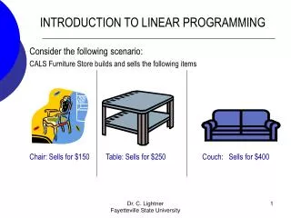
An Example of a LP • Giapetto’s woodcarving manufactures two types of wooden toys: soldiers and trains. How many of each type to produce? Constraints: • 100 finishing hour per week available • 80 carpentry hours per week available • produce no more than 40 soldiers per week • Objective: maximize profit? Minimize cost?
An Example of a LP (cont.) Linear Programming formulation: Maximize z = 3x1 + 2x2(Obj. Func.) subject to 2x1 + x2 100 (Finishing constraint) x1 + x2 80 (Carpentry constraint) x1 40 (Bound on soldiers) x1 0 (Sign restriction) x2 0 (Sign restriction)
Assumptions of Linear Programming • Proportionality Assumption • Contribution of a variable is proportional to its value. • Additivity Assumptions • Contributions of variables both in the objective and in the constraints are independent of the values of the other variables. No interactions between the variables. • Divisibility Assumption • Decision variables can take fractional values. • Certainty Assumption • Each parameter is known with certainty.
Transportation Problem • The Brazilian coffee company processes coffee beans into coffee at m plants. The production capacity at plant i is ai. • The coffee is shipped every week to n warehouses in major cities for retail, distribution, and exporting. The demand at warehouse j is bj. • The unit shipping cost from plant i to warehouse j is cij. • It is desired to find the production-shipping pattern xij from plant i to warehouse j, i = 1, .. , m, j = 1, …, n, that minimizes the overall shipping cost. • What is Xij? Produced? Shipped? • Why not consider production and shipping together? • Why not maximize profit?
Static Workforce Scheduling • Number of full time employees required on different days of the week are given below. • Each employee must work five consecutive days and then receive two days off. • The schedule must meet the requirements by minimizing the total number of full time employees. • Decision variable?
Cutting Stock Problem • A manufacturer of metal sheets produces rolls of standard fixed width w and of standard length l. • A large order is placed by a customer who needs sheets of width w and varying lengths. He needs bi sheets of length li, i = 1, …, m. • The manufacturer would like to cut standard rolls in such a way as to satisfy the order and to minimize the waste. • Since scrap pieces are useless to the manufacturer, the objective is to minimize the number of rolls needed to satisfy the order. • Decision variable? • Objective ?
Multi-Period Workforce Scheduling • Requirement of skilled repair time (in hours) is given below. • At the beginning of the period, 50 skilled technicians are available. • Each technician is paid $2,000 and works up to 160 hrs per month. • Each month 5% of the technicians leave. • A new technician needs one month of training, is paid $1,000 per month, and requires 50 hours of supervision of a trained technician. • Decision variable(s)? Objective?
Feed mix problem • An agricultural mill manufactures feed for chickens. This is done by mixingseveral ingredients, such as corn, limestone, or alfalfa. • The mixing is to be done insuch a way that the feed meets certain levels for different types of nutrients (mins and maxs), suchas protein, calcium, carbohydrates, and vitamins. • To be more specific, supposethat n ingredients y = 1,..., n and m nutrients / = 1,..., m are considered. • Total amount of feed must be equal to a certain value • Objective? Decision variables?
Solution: Transportation Problem Decision Variables: xijp: amount of product p shipped from plant i to warehouse j Formulation: Minimize z = subject to <= ai, i = 1, … , m bj, j = 1, … , n xij 0, i = 1, … , m, j = 1, … , n
Solution: Static Workforce Scheduling LP Formulation: Min. z = x1+ x2 + x3 + x4 + x5 + x6 + x7 subject to x1 + x4 + x5 + x6 + x7³17 x1+ x2 + x5 + x6 + x7³13 x1+ x2 + x3 + x6 + x7 ³15 x1+ x2 + x3 + x4 + x7³19 x1+ x2 + x3 + x4 + x5³14 x2 + x3 + x4 + x5 + x6³16 x3 + x4 + x5 + x6 + x7³11 x1, x2, x3, x4, x5, x6, x7³ 0
Solution: Multiperiod Workforce Scheduling Decision Variables: xt: number of technicians trained in period t yt: number of experienced technicians in period t Formulation: Minimize z = 1000(x1 + x2 + x3 + x4 + x5) + 2000(y1 + y2 + y3 + y4 + y5) subject to 160y1 - 50 x1³ 6000 y1 = 50 160y2 - 50 x2³ 7000 0.95y1 + x1 = y2 160y3 - 50 x3³ 8000 0.95y2 + x2 = y3 160y4 - 50 x4³ 9500 0.95y3 + x3 = y4 160y5 - 50 x5³11000 0.95y4 + x4 = y5 xt, yt³ 0, t = 1, 2, 3, … , 5
Cutting Stock Problem • We want certain number of specific length pieces that must be cut out of standard length pieces. • Given a standard sheet of length l, there are many ways of cutting it. Each such way is called a cutting pattern. • The jth cutting pattern is characterized by the column vector aj, where the ith component, namely, aij, is a nonnegative integer denoting the number of sheets of length li in the jth pattern. • Note that the vector aj represents a cutting pattern if and only if i=1,n aijli l for patter j where each aij is a nonnegative number. • Example; let l=7 feet and we want to have pieces with lengths 2, 3, and 5. • Possible patterns (2x1, 5x1), (2x3), (3x2), (2x2,3x1) • Objective? Decision varb.?
Solution:Cutting Stock Problem (contd.) Formulation: xi: Number of sheets cut using patter j. There are n possible patterns, m different lengths to produce. Minimize j=1,n xi subject to j=1,n aij xj bi for each i = 1, …, m xj 0 j = 1, …, n xjinteger j = 1, …, n
Solution:Cutting Stock Problem (contd.) Formulation: Let l = 7, and type 1, type 2 and type 3 sizes demanded are 2, 3, and 5 with b1=10, b2=4, b3=3. possible patterns: j 3 2 0 1 i 0 1 2 0 0 0 0 1 Min. z = x1+ x2 + x3 + x4 subject to 3x1+2 x2 + x4 10 x2 + 2x3 4 x4 3 xj integer j = 1, …, 4
Solution:Cutting Stock Problem (contd.) Formulation: Let l = 7, and type 1, type 2 and type 3 sizes demanded are 2, 3, and 5 with b1=10, b2=4, b3=3. possible patterns: j 3 2 0 1 i 0 1 2 0 0 0 0 1 Min. z = x1+ x2 + x3 + x4 subject to 3x1+2 x2 + x4 10 x2 + 2x3 4 x4 3 xj integer j = 1, …, 4
Solution: Feed mix problem • Decision variable; Let the amount of ingredient j to be used be xj. • Let aij be the amount of nutrient ipresent in a unit of ingredient j • Acceptable lower and upper limits ofnutrient j in a unit of the chicken feed are lj‘ and uj’, respectively. (There are also upper limits on ingredients available, represented by uj’s.) • Objective; Minimize total cost
Modeling issues • Minimize/Maximize absolute value => For maximimization problems multiply objective with -1 and turn them into minimization problem
Modeling issues X,Y >=0
Modeling issues • Fixed charge problem: Cost function with a fixed part
Modeling issues Decision variables
Modeling issues • Either-or constraints:
Modeling issues Decision variables
Modeling issues Constraints What M1 should we use?
Modeling issues • If-then constraints
Modelling issues n out of k constraints must hold • 1 out of k constraints must hold
Modelling issues • Reconsider the example on Gandhi clothing company with the following additional information; • Current clothing supplier (supplier 1) can supply 160 sq-yard per week. Lets say that there are two additional suppliers; • Supplier 2 can supply clothing minimum 100 and maximum 200 sq-yard per week and supplier 3 can supply between 150 and 300 sq-yard per week. • That is supplier 2 and 3 require a minimum purchase in addition to a maximum. Company must work with only one supplier due to logistical reasons. How can we model the same problem with three suppliers option?
Geometric Solution • Steps of the geometric solution • Determine and draw the feasible region • Draw the c vector • Draw the iso cost lines (perpendicular to c vector) • Find the last point(s) that iso-cost lines touch the feasible region, when we move towards direction of –c (in minimization). This point (or points) is the optimal solution.