Download

1 / 44
540 likes | 945 Views
Gregorio Gomez Robert Sauermann Ben Lynton. Heat waves. Presentation Outline. Introduction: What is a heat wave? 2010 Russian Heat Wave Dole et al. (2011): Natural Variability & “Omega” Blocking Rahmstorf & Coumou (2011): Warming & Frequency Otto et al. (2012): Reconciling 1 & 2

E N D
Gregorio Gomez Robert Sauermann Ben Lynton Heat waves
Presentation Outline Introduction: What is a heat wave? 2010 Russian Heat Wave Dole et al. (2011): Natural Variability & “Omega” Blocking Rahmstorf & Coumou (2011): Warming & Frequency Otto et al. (2012): Reconciling 1 & 2 Samenow article (2012): Public Perception Debate: Has global warming had an effect on heat waves? http://www.youtube.com/watch?v=hl9WYhYJjqQ
Historical Heat Waves 1858, London’s Great Stink 1936, North America Great Depression, drought, dust storms Record temperatures in 12 states, clearing 120oF 5,000 US and 1,100 Canadian deaths 1995, Chicago 106oF = average Arizona temperatures 700 deaths in 5 days, infrastructure break down 2003, Western Europe Hottest summer since 1500 A.D. 40,000 deaths + forest fires, glacier floods, crop destroyed History Channel: http://www.history.com/news/history-lists/heat-waves-throughout-history
2010 Russian Heat Wave slide 5: note that this graph (and many of the other graphs) are actually temperature anomalies, which the authors do not say in their caption. Recommend replacing their y-axis with one that correctly describes the data 55,000 deaths 25% annual crop production decrease 15 billion USD loss to the Russian economyhttp://www.youtube.com/watch?v=eCb0pNY5jeE Temperature Anomalies (°C) Off of average temperature 11/1/09-10/31/10 Average climatological seasonal cycle Above average temperature Below average temperatures *National Climatic Data Center: Global Summary of the Day
What is a Heat Wave? • The World Meteorological Organization considers a climatic event a heat wave if the local maximum daily temperature exceeds the historical average by 5°C for 5 consecutive days. • Heat “Wave/Dome” • High pressure in mid/upper atmosphere (5km) • diverts jet stream • stifles circulation • traps heat on surface • Magnified by sun angle,clear skies, and drought (latent heat) slide 6: remember that you'll want to be able to explain the heat dome, so make sure you all understand it!
slide 7: 'comparison' is showing a change in shape (there's a change in mean and I believe a change in the skew) -- would label correctly, or not include. Understanding Statistics: Mean and Variability An increase in the mean raised heat wave frequency Increases in the variability raise hot and cold event frequencies Changes in mean or variability affect heat wave frequency differently
1. Dole et al. (2011) Randall Dole • Fellow of the American Meteorological Society • Division Director for the CIRES and IPCC member
slide 9: generally recommend not presenting the conclusions first, rather present motivation and methods, and we'll talk through the conclusions by looking at figures. Folks won't necessarily understand the conclusions bullet points until we've talked about the paper Motivation Cause of 2010 Russian Heat Wave: What were the primary causes for 2010 Western Russian heat wave? Predictability of Russian 2010 Heat Wave: Based on natural and human forcings and observed regional climate trends, could the heat wave have been predicted?
slide 10: 'data experiments' doesn't make a lot of sense -- we'd typically say 'data analysis', and you're actually just presenting the datasets they are using. What is the purpose of your underlines? While helpful for highlighting things, they seem to highlight words that are not all in the same category (i.e. frequency/variability vs boundary conditions) Methodology: Data & Models • Data • Observations • Western Russian mean July temperatures • Extreme temperature event frequency/variability • Datasets • NOAA, GHCN, NASA, GISTEMP • Model Experiments • Simulations to observe trends in heat wave frequency • IPCC CMIP3 model • Evaluate potential effects of July 2010 boundary conditions • AM2.1, MAECHAM5 • Future global warming effects on heat waves • IPCC CMIP3 model
Western Russia Mean July Temperatures since 1880 Western Russia July temp change = -0.1°C / 130yrs =.0008 °C/yr = July Mean T2009 – July Mean T1880 (°C/130yrs) Western Europe Large temp change (Recall 2003 heat wave) No significant temperature change in Western Russia from 1880-2009 Mean regional July temp trend unlikely to have caused 2010 heat wave
slide 14: recommend 'western russia does not show an increase in temperature variability' or similar for title Western Russia Shows No Increase In Temperature Variability 2010 ##: year of top 10 (+) anomaly (+) anomalies (-) anomalies Mean Temp 1880-2009 Light Grey: simulated temperature anomalies (normalized) Dark Grey: simulated temperature anomalies (non-normalized) Both are based on 22 CMIP3 model simulations No observable trends in Western Russia temperature extremes Temperature variability trend unlikely to have caused 2010 heat wave
Statistical Summary: neither mean nor variability explain 2010 heat wave 1880-1944 1945-2009 1880-1944 1945-2009 • No significant difference in Western Russia temp mean over last 65 years than previous 65 years (t-test) • No significant difference in Western Russia temp variability over last 65years than previous 65years (F-Test) “no statistically significant long-term change is detected in either the mean or variability of Western Russia July temperatures”
“Omega” Blocking Pattern Pressure: Low-High-Low • High pressure over large latitude Disturbs Jet Stream • Difficult for air flow to move from west to east over high pressure hump traps heat Region under Ω Block • dry weather, light wind Ω troughs • Rain and clouds • Omega Blocking is a common cause of heat waves
Typical Western Russia Heat Wave Conditions • Top 10 Composite • Height of pressure bar anomalies off of 5000m • (in 10s of meters) ##: year of top 10 (+) anomaly • Temp anomalies off of local average surface temperature (°C) • Top 10 Heat Waves exhibit classic “omega” blocking pattern
Comparing 2010 with Top 10 • Top 10 Composite • 2010 Heat Wave • Height of pressure bar anomalies off of 5000m • (in 10s of meters) • Height of pressure bar anomalies off of 5000m • (in 10s of meters) • Temp anomalies off of local average surface temperature in (°C) • Temp anomalies off of local average surface temperature (°C) • 2010 Heat Wave Consistent with Top 10 Composite • 2010 Heat Wave exhibits classic “omega” blocking
slide 20: would make title more specific, as we're specifically testing if the predictability can come from boundary conditions. Moreover, the Blocking Pattern was not Predictable MAECHAM5 ~ Boundary Conditions Forcing GDFL AM2.1 ~ NOAA CFS July 2010 climate conditions GDFL AM2.1 and MAECHAM5 • natural and human forcings • e.g. SSTs, arctic sea ice 50-member ensemble • Inconsistent with “Ω”blocking Single Model Simulation • Qualitatively similar to observations • Reflect internal atmospheric variabilityrather than systematic response to boundary conditions • Height of pressure bar anomalies off of 5000m • (in 10s of meters) • Temperature anomalies off of local average surface temp in (°C) • Height of pressure bar anomalies off of 5000m • (in 10s of meters) • Temperature anomalies off of local average surface temp in (°C) • Boundary Conditions could not predict 2010 Blocking Pattern
Not mean shift, Not increased variability, Not Boundary Conditions 2010 Heat Wave not predictable, and likely due to natural variability
Probability of Future Heat Waves on Earth % of 22 CMIP3 models that simulate ≥ 10% probability of heat wave occurrence CMIP3 models show increase in heat wave frequency, with uncertain timing due to sensitivity in greenhouse gas concentration predictions • Models predict global increase in the probability of future heat waves
slide 9: generally recommend not presenting the conclusions first, rather present motivation and methods, and we'll talk through the conclusions by looking at figures. Folks won't necessarily understand the conclusions bullet points until we've talked about the paper Conclusions Cause of 2010 Russian Heat Wave: Internal atmospheric variability created an “omega” blocking period which caused the heat wave. Predictability of 2010 Russian Heat Wave: The 2010 Western Russian heat wave could not have been predicted as there have not been observed changes in mean temperatures or extreme temperature variability, and boundary conditions could not have predicted the ‘omega’ blocking event.
2. Rahmstorf & Coumou (2011) • Stefan Rahmstorf: Paper 2 • German climate change advisory council member • Author of paleo-climate chapter in 4th IPCC report Dim Coumou: Paper 2 • PotsdamInstitute of Climate Impact Research member
Motivation • Heat Wave Frequency : How do warming trends influence the expected number of record breaking and threshold breaking heat waves? • Cause of Moscow Heat Wave: What is the probability that local warming trends caused the 2010 Moscow Heat Wave?
Methodology • Data: - NASA Goddard Institute for Space Studies (GISS) annual global temperature (0.09°C variability, + 0.70°C / last 100 years) - Moscow Weather Station mean July temperature (1.7°C variability, + 1.8°C / last 100 years) • Simulations / Calculations: 1. Generated Gaussian distributions of stationary climate, linearly increasing climate, and non-linearly increasing climate 2. Applied theoretical results to GISS data and Moscow data 3. Calculated expected probability and number of heat records in past decade
slide 7: 'comparison' is showing a change in shape (there's a change in mean and I believe a change in the skew) -- would label correctly, or not include. Understanding Statistics: Mean and Variability An increase in the mean raised heat wave frequency Increases in the variability raise hot and cold event frequencies Changes in mean or variability affect heat wave frequency differently
Calculating theoretical probability of record events Stationary Climate (blue) Non-stationary Climate • Probability of record = (1/n) • (n = # of data points) • Defined as a climate with no long term deviation from T̅ • Results from either shifting long term mean (T̅), changing the distribution of T, or both • Linear warming trend → approx. linear increase in expected probability of record events Stationary v. Non-stationary probability trends • More extreme events are expected in Non-Stationary climates (+ or -)
Monte-Carlo simulations match actual temp distributions Simulated Gaussian noise v. actual temperatures • Simulatednoise with stationary trend • Simulated noise with ↑ linear trend = 0.078/year • Simulated noise with ↑ non-linear smoothed NASA GISS trend • Normalized global annual NASA GISS temp. + non linear trend (1911 – 2010) • Normalized Moscow station July temp. + non linear trend (1911 – 2010) • Normalized non-linear trends are the best approx. of actual conditions
Increases in warming lead to more Unprecedented and Threshold Breaking Events Unprecedented Events Threshold Breaking Events • Approx. linear increase • Non-linear increase Exp. Records v. warming trend Exp. Events v. warming trend (.078,1.4) (.078,~7) ±3 Warm events increase # Record events in past decade # threshold breaking events in past decade ±4 (.078,~3) Cold events approach 0 Observed trend (GISS) Observed trend (GISS) • Both record frequency and threshold breaking frequency • increase with warming, but at different rates
Smooth non-linear climate trend is best model of both Global and Moscow temperatures • To accept a non-linear trend in temperature, temperature deviations (residuals) should exhibit near Gaussian distribution and no autocorrelation NASA GISS (1911 – 2010) Moscow Station (1911 – 2010) • SDG = .088°C • Autocorrelation: r = .17 • SDMS = 1.71°C (19x SDG) • Autocorrelation: r = -0.04 • Noise is not exactly Gaussian but is stationary and reasonably close
Results of applying Monte-Carlo simulations to increasing GMT observed in NASA GISS data Linear trend (100 yr) Percentage of simulations v. # of expected heat extremes (100 year linear trend) • Predicted extremes = 1.4 • Trend = .0078°C/yr • Note: Increased inter-annual variability → increased # of extreme events, but decreased # of unprecedented events Linear trend (30 yr) 13% 19% • Predicted extremes = 2.4 • Trend = .017°C/yr 28% 39% Non-Linear trend • Predicted extremes = 2.8 *predicated extremes for 2000-2010 • If a non-linear trend (or recent linear trend) is used, more • Global unprecedented heat extremes are expected
Results of applying Monte-Carlo simulations to increasing July Moscow temperatures • Given linear warming trend of .011/yr, sim predicts .29 unprecedented heat extremes in past decade • Given non-linear warming trend, simpredicts .85 unprecedented heat extremes in past decade • In stationary climate .105 unprecedented heat extremes are expected Predicted Record Heat Extremes In Stat. & Non-Stat. Climates Expected Unprecedented Heat Extremes / Decade Replace lin warm trend w/ ratio Blue = Red = Non linear Moscow Trend • If a non-linear trend (or recent linear trend) is used, more • Global unprecedented heat extremes are expected
Increased probability of Russian heat record in last decade is attributable to warming trend (Rnon – Rstat) / Rnon = Prec • Rahmstorf and Coumou find post 1980 warming trend most relevant • Relies on notion that warming trends will directly increase the number of record heat waves (i.e. perfect causality) Determines probability that the 2010 heat record is result of warming by measuring % diff. between stationary and non stationary predictions Linear Non-Linear Non-Linear (2010 omitted) • Rnon = .29 • Prec = 64% • Rnon = .85 • Prec = 88% • Rnon = .47 • Prec = 78% • Prec= 80% (1880 – 2009) • Concludes w/ 80% prob. the Moscow Heat Wave is a result of warming
Potential influence of Moscow urban heat island • Note their previous analysis does not address causes of warming trend • Claim1/3 of Moscow warming due to local urban heat island effect (2°C / last 30 yrs in city, 1.4°C / last 30 yrs in region – 2X Global avg) • Rest of warming result of continental warming due to ↑ Global temp • Western Russia is similar to other continental interiors, and models predict similar results in greenhouse gas forced scenarios (cites 2007 IPCC report) Microwave sounding Satellite Data Red = Moscow region Blue = Moscow Station Temp Anomaly (°C) Years (1979 – 2009) • Local warming trend observed in Western Russia is • largely a result of anthropogenic greenhouse warming
Conclusions • Rising mean annual global temperatures and mean July Moscow temperatures have increased the expected probability of an unprecedented heat wave • Statistical models show an approximate 80% probability that the 2010 Russian heat wave would not have occurred without global warming • The Local warming trend observed in Western Russia is largely a result of anthropogenic greenhouse warming
3. Otto et al. (2012) • Friederike Otto • Research fellow at the ECI global climate science program • Work primarily based on improving climate models with emphasis on extreme events
Motivation Reconciling Paper 1 & 2: Do Dole et al.(2011) & Rahmstorf and Coumou (2011) really contradict each other? Global Warming’s role in 2010 Russian Heat Wave: “Whether and to what extent this event is attributable to anthropogenic climate change?”
Methodology Ensemble Simulations Definition: The results of mass model simulations using various different initial conditions are compiled to create a probability function with which observed data can be analyzed. Applicability: Climate models rely on a vast number of variables and so one stand alone simulation (especially for the less complex models) can be unreliable. Otto et al., ran simulations for years with high resolutions that would lead to the best data to base their findings off of.
Modelled and Observed Temperature Anomalies • 2010 heat wave was far above the 95thquantile which seen as an extreme anomaly. • Warming in Western Russia is 1.9±0.8 times that of the global trend. • The function creating the red line is assuming that the probability density function has not changed shape but rather it’s shifted to a higher mean. Normalized Temp Anomaly • The 2010 heat wave is far above any reasonable projections
Using Simulated 500 hPaAltitudes to Test Model Accuracy • Otto et al., test the accuracy of their model by comparing simulated 500 hPa altitudes in (a) to observed reanalysis data in (b) • Part (b) contains more variability than (a) due to its data set being far smaller that that of the model. • Modelled vs. Observed 500 hPa Anomaly Altitudes • Height anomalies (km) • off of height of 5km • Comparing their model to observations lends credibility to its accuracy
Reasonably strong correlation between 500 hPa altitudes and mean July temperatures • Scatter plot of mean Russian temperatures Vs 500 hPa mean geopotential heights. • Corrected for bias and including a line representing a 1 to 1 relationship, the second graph shows that their regression pattern is promisingly accurate. 2010 Heat Wave 2010 heat wave Temp°C • The 2010 heat wave follows the 1 to 1 trend • between geopotential height and temp.
Comparing Conclusions from Paper 1 & 2 Return Time Vs. Magnitude • Return time is a theoretical measure of how often an event of a particular magnitude will occur. • They used mean temperatures from the 1960’s and the 2000’s to produce two different curves illustrating the difference in heat wave frequency. °C +1°C 33 (Years) • The figure suggests that both high natural variability and increased heat wave frequency could have caused the 2010 heat wave.
Conclusions • Paper 1 claims the heat wave could not have been anticipated because it was caused principally by natural variability in the West Russian climate. • Paper 2 fits a trend to Russian temperatures to show that the recent warming has raised the predicted frequency of extreme events. • Having checked empirical data and conducted numerous simulations, both of the conclusions proposed by the different authors could be true. • Analysis of large Ensemble Simulations suggest that it is possible for the 2010 heat wave to have been caused by both natural variability or by increased risk caused by a local warming trend.
Epic March — The Washington Post (2012) • Jason Samenow: • Weather editor for the Washington Post • Chief Meteorologist for the Capital Weather Gang Blog Record Highs in Midwest, Great Lakes, Northeast Link to Global Warming? • U of Utah, TWC representatives attribute global warming • Accuweather representatives ask for more data • Public opinion is varied, yet potentially influential