Download
1 / 22
220 likes | 346 Views
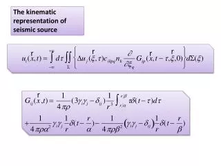
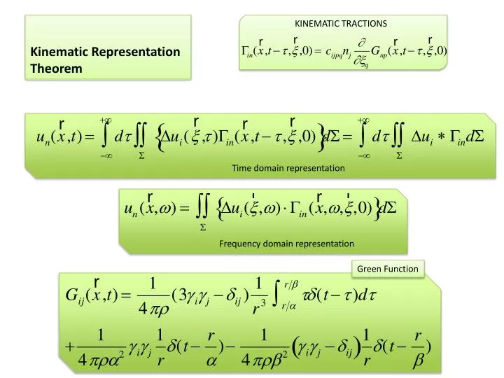
Kinematic Representation Theorem. KINEMATIC TRACTIONS. Time domain representation. Frequency domain representation. Green Function. Far Field case. Near Field vs Far Field f = 1 Hz, r = 6 km f = 0.01 Hz, r =300 km, c= b =3.5 Km/s c= b =3.0 Km/s. In the Far Field we have r >> l

E N D
Kinematic Representation Theorem KINEMATIC TRACTIONS Time domain representation Frequency domain representation Green Function
Far Field case • Near Field vs Far Field f = 1 Hz, r = 6 km f = 0.01 Hz, r =300 km, c=b=3.5 Km/s c=b=3.0 Km/s In the Far Field we have r >> l If Thus we have the far field – far source (point source) If Thus we have the far field – near source (extended source)
Numerical complete solution for elastodynamic Green Function • Equation of motion m = 0,±1,±2,±3,etc…. Jm is the Bessel of order m We develop the solution in a cylindrical coordinate system (r, f, z), in which z is the vertical axis. The elastic parameters vary only on the vertical axis z. The dependence on r and f results only superficial harmonics, which are orthogonal vectors
Development of a generic vector in orthogonal functions A generic vector that is a function of the variable r and f, can be written in terms The Fourier transform of its components can be written as
Discrete wavenumber method • Solution has the form The solution is expressed in terms of Bessel functon
WavesAmplitude Attenuation • Wave amplitudes decrease during propagation • Causes: • geometrical spreading (elastic) • Reflection and transmission coefficients • scattering (elastic) • Impedance contrast (elastic) • attenuation (anelastic)
Geometrical spreading of four rays at two different values of travel time (to, t) THE GEOMETRICAL SPREADING ds(to) and ds(t) are the two elementary surfaces describing the section of the ray tube on the wave front at different times. The geometrical spreading factor in inhomogeneous media describes the focusing and defocusing of seismic rays. In other words, the geometrical spreading can be seen as the density of arriving rays; high amplitudes are expected where rays are concentrated and low amplitudes where rays are sparse. The focusing or defocusing of the rays can be estimated by measuring the areal section on the wave front at different times defined by four rays limiting an elementary ray tube. Each elementary area at a given time is proportional to the solid angle defining the ray tube at the source , but the size of the elementary area varies along the ray tube.
Reflection & Transmission Coefficient The reflection coefficient is used in physics and electrical engineering when wave propagation in a medium containing discontinuities is considered. A reflection coefficient describes either the amplitude or the intensity of a reflected wave relative to an incident wave. The reflection coefficient is closely related to the transmission coefficient. Reflection & transmission coeff.
Some properties See Aki & Richards (2002) chapter 5 for an extended presentation of R and T for more realistic waves
Impedance contrast • The impedance that a given medium presents to a given motion is a measure of the amount of resistance to particle motion. The product of density and seismic velocity is the acoustic impedance, which varies among different rock layers, commonly symbolized by Z. The difference in acoustic impedance between rock layers affects the reflection coefficient. For a SH wave
Anelastic Attenuation – the Quality factor If a volume of material is cycled in stress at a frequency w, a dimensionless measure of the anelasticity (internal friction) is given by where E is the peak strain energy stored in the volume and DE is the energy lost in each cycle. We can transform this in terms of the amplitudes E = A2, If we consider a damped harmonic oscillator, we can write where wo is the natural frequency and g is the damping factor
Body wave attenuation Body wave attenuation is commonly parameterized through the parameter t*
Comportamento anelastico: anisotropia Olivine is seismically anisotropic (mantello) Courtesy of Ben Holtzman
Comportamento anelasticoAnisotropia nel mantello Animation from the website of Ed Garnero • SKS splitting
Comportamento anelasticoAnisotropia nel mantello • SKS splitting Fenomeno della birifrangenza
SKS phases radial comp. transversal comp. fast fast delay time slow slow Courtesy of Ben Holtzman