Download
1 / 22
220 likes | 228 Views
Grid-based Map Analysis Techniques and Modeling Workshop. Part 1 – Maps as Data Part 2– Surface Modeling Part 3 – Spatial Data Mining Part 4 – Spatial Analysis Suitability mapping Measuring effective distance/connectivity Visual exposure analysis Analyzing landscape structure

E N D
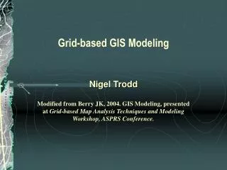
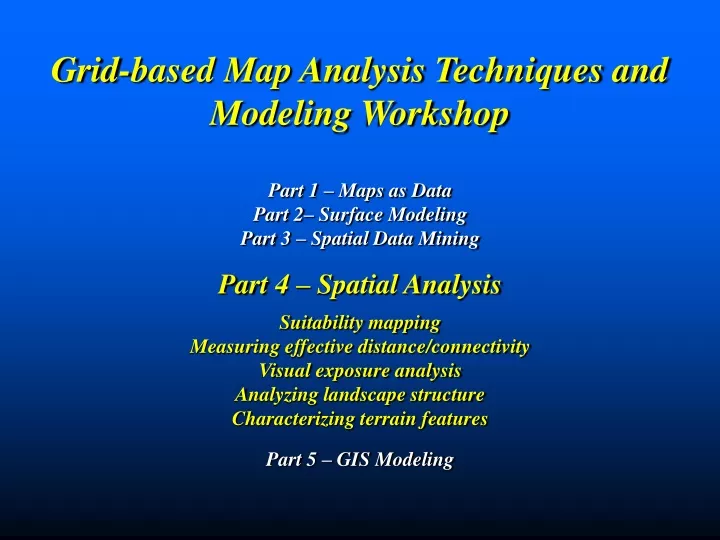
Grid-based Map Analysis Techniques and Modeling Workshop Part 1 – Maps as Data Part 2– Surface Modeling Part 3 – Spatial Data Mining Part 4 – Spatial Analysis Suitability mapping Measuring effective distance/connectivity Visual exposure analysis Analyzing landscape structure Characterizing terrain features Part 5 – GIS Modeling
Grid-Based Map Analysis • Surface Modelingmaps the spatial distribution and pattern of point data… • Map Generalization— characterizes spatial trends (e.g., titled plane) • Spatial Interpolation— deriving spatial distributions (e.g., IDW, Krig) • Other— roving window/facets (e.g., density surface; tessellation) • Data Mininginvestigates the “numerical” relationships in mapped data… • Descriptive— aggregate statistics (e.g., average/stdev, similarity, clustering) • Predictive— relationships among maps (e.g., regression) • Prescriptive— appropriate actions (e.g., optimization) • Spatial Analysisinvestigates the “contextual” relationships in mapped data… • Reclassify— reassigning map values (position; value; size, shape; contiguity) • Overlay— map overlay (point-by-point; region-wide; map-wide) • Distance— proximity and connectivity (movement; optimal paths; visibility) • Neighbors— ”roving windows” (slope/aspect; diversity; anomaly) (Berry)
Evaluating Habitat Suitability Generating maps of animal habitat… Manual Map Overlay Ranking Overlay Rating Overlay Assumptions– Hugags like gentle slopes, southerly aspects and lower elevations (Berry)
Conveying Suitability Model Logic Calibrate Algorithm gentle slopes Elevation Slope Slope Preference Bad 1 to 9 Good Weight southerly aspects Elevation Aspect Aspect Preference Bad 1 to 9 Good Habitat Rating Bad 1 to 9 Good lower elevations Elevation Elevation Preference Bad 1 to 9 Good Habitat Rating 0= No, 1 to 9 Good Base Maps Derived Maps Interpreted Maps Solution Map Fact Judgment Covertype Water Mask 0= No, 1= Yes Constraint Map (Berry) (See map Analysis, “Topic 22” for more information)
Extending Model Criteria (Times 10) (1) (1) forests Forests Forest Proximity Forest Preference Bad 1 to 9 Good (10) water Water Water Proximity Water Preference Bad 1 to 9 Good (10) gentle slopes Elevation Slope Slope Preference Bad 1 to 9 Good southerly aspects Elevation Aspect Aspect Preference Bad 1 to 9 Good Habitat Rating Bad 1 to 9 Good lower elevations Additional criteria can be added… Elevation Elevation Preference Bad 1 to 9 Good • Hugags would prefer to be in/near forested areas • Hugags would prefer to be near water • Hugags are 10 times more concerned with slope, forest and water criteriathan aspect and elevation (Berry)
Establishing Distance and Connectivity (digital slide show DIST) (Berry)
Point Orthogonal distances are the same as calculated by the Pythagorean Theorem and align with a circle of a given radius… …other distances contain slight “rounding” errors Proximity Ripples for a large steps away from a starting location align fairly well with an exact circle… …but poorly align for small steps Points Lines Polygons …an excellent technique for generating simple and effective proximity surfaces respecting absolute and relative barriers to movement from sets of points, lines and polygons (impossible to do with the Pythagorean Theorem ) Grid-based Simple Proximity Surfaces (Berry)
Calculating Effective Distance (Demo) Simple Proximity …as the crow flies …the Splash Algorithm is like tossing a rock into a still pond with increasing distance rings that abut and bend around absolute and relative barriers 0= not able to cross 2= two min. to cross 7 = seven min. to cross Effective Proximity …as the crow walks (Berry)
Generating an Effective Travel-time Buffer • superimposition of an analysis grid over the area of interest • “burns” the store location into its corresponding grid cell • “burns” primary and residential streets are identified • travel-time buffer derived from the two grid layers (Berry)
…SPREADing from multiple locations identifies catchment areas– locations closest to starting locations …what do you think the ridges represent? Travel-Time Connectivity …increasing distance from a point forms bowl-shaped accumulation surface …steepest downhill path identifies the optimal path– wave front that got there first. (Berry)
…increasing distance from a point forms bowl-shaped accumulation surface Simple distance – symmetrical bowl Absolute barrier – abrupt pillars Relative barrier – gradual humps …subtracting two proximity surfaces identifies relative advantage Zero – equidistant Sign – which has the advantage Magnitude – strength of advantage …what would get if you added the two surfaces? Accumulation Surface Analysis (See Map Analysis, “Topic 5” and “Topic 17” for more information) (Berry)
Seen if new tangent exceeds all previous tangents along the line of sight— At <Viewer_heightValue> Thru <Screens_heightMap>) Onto <Target_heightMap> …like measuring proximity, it starts somewhere (starter cell) and moves through geographic space by steps (wave front) evaluating whether the moving tangent is beat— …if so, the location is marked as “seen” and its tangent is assigned as the one to beat Radiate – visual exposure is calculated bay a series of “waves” that carry the tangent to beat. Simply – viewshed Completely – number of “viewers” that see each location Weighted – viewer cell value is added Establishing Visual Connectivity (Berry)
Visual exposure identifies how many times each map location is seen from a set of viewer locations Calculating Visual Exposure (# Times Seen) (Berry)
A visual exposure map identifies how many times each location is seen from an “extended eyeball” composed of numerous viewer locations (road network) Visual Exposure from Extended Features (Berry)
Different road types are weighted by the relative number of cars per unit of time …the total “number of cars” replaces the “number of times seen” for each grid location Weighted Visual Exposure (Sum of Viewer Weights) (See Map Analysis, Topic 15, “Deriving and Using Visual Exposure Maps” for more information) (Berry)
Calculating Visual Exposure (Demo) Viewshed …as the crow sees (seen or not seen) Visual Exposure …as the flock sees (# times seen) Weighted Visual Exposure …as the flock sees (not all in the flock are the same) (Berry)
Weighted visual exposure map for an ongoing visual assessment in a national recreation area— the project developed visual vulnerability maps from the reservoir in the center of the park and a major highway running through the park. In addition, aesthetic maps were generated based on visual exposure to pretty and ugly places in the park Real-World Visual Analysis (Senior Honors Thesis by University of Denver Geography student Chris Martin, 2003) (Berry)
Neighborhood Techniques (Covertype Diversity Map) …a DIVERSITY map indicates the number of different map values (categories) that occur within a window… e.g., cover types As the window is enlarged, the diversity generally increases (Berry)
Neighbor Techniques (Demo) • SCAN Covertype diversity within 3 for Cover_diversity3 • SCAN Slope coffvar with 2 for Roughness • SCAN Housing total with 5 for Housing_density • RENUMBER Housing_density for High_hdensity • assign 0 to 0 thru 15 assign 1 to 15 thru 50 • COMPOSITE Districts with Housing_density average • for Districts_HDavg Housing Density by Districts Average housing density for each district (Berry)
Neighborhood Variability (See MapCalc Applications, “Assessing Cover Type Diversity and Delineating Core Area” and “Assessing Covertype Diversity” for more information) (Berry)
Size of individual patches is an important first-order assessment of landscape structure The amount and type of edge tracks the nature of the patch interface P/A ratio tracks patch shape… boundary irregularity (digital slide show FRAG) (digital slide show NN_statistics) See http://www.innovativegis.com/products/fragstatsarc/index.html for more information Spatial Analysis of Landscape Structure Area Metrics (6), Patch Density, Size and Variability Metrics (5), Edge Metrics (8), Shape Metrics (8), Core Area Metrics (15), Nearest Neighbor Metrics (6), Diversity Metrics (9), Contagion and Interspersion Metrics (2) …59 individual indices(US Forest Service 1995 Report PNW-GTR-351) For example, • Area Metrics …Area per patch • Shape Metrics …Shape Index per patch • Edge Metrics …Edge Contrast per patch (Berry)
Grid-Based Map Analysis • Surface Modelingmaps the spatial distribution and pattern of point data… • Map Generalization— characterizes spatial trends (e.g., titled plane) • Spatial Interpolation— deriving spatial distributions (e.g., IDW, Krig) • Other— roving window/facets (e.g., density surface; tessellation) ...Whew!!! • Data Mininginvestigates the “numerical” relationships in mapped data… • Descriptive— aggregate statistics (e.g., average/stdev, similarity, clustering) • Predictive— relationships among maps (e.g., regression) • Prescriptive— appropriate actions (e.g., optimization) • Spatial Analysisinvestigates the “contextual” relationships in mapped data… • Reclassify— reassigning map values (position; value; size, shape; contiguity) • Overlay— map overlay (point-by-point; region-wide; map-wide) • Distance— proximity and connectivity (movement; optimal paths; visibility) • Neighbors— ”roving windows” (slope/aspect; diversity; anomaly) (Berry)