Download
1 / 37
380 likes | 398 Views
Traditional GIS. Spatial Analysis. Forest Inventory Map. Erosion Potential (Surface). Points, Lines, Polygons Discrete Objects Mapping and Geo-query. Cells, Surfaces Continuous Geographic Space Contextual Spatial Relationships. Spatial Statistics. Traditional Statistics.

E N D
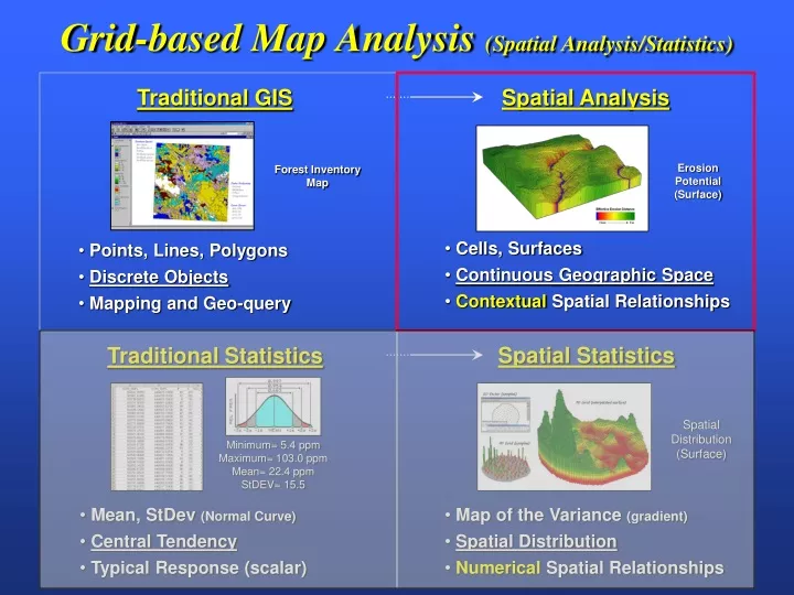
Traditional GIS Spatial Analysis Forest Inventory Map Erosion Potential (Surface) • Points, Lines, Polygons • Discrete Objects • Mapping and Geo-query • Cells, Surfaces • Continuous Geographic Space • Contextual Spatial Relationships Spatial Statistics Traditional Statistics Spatial Distribution (Surface) Minimum= 5.4 ppm Maximum= 103.0 ppm Mean= 22.4 ppm StDEV= 15.5 • Mean, StDev (Normal Curve) • Central Tendency • Typical Response (scalar) • Map of the Variance (gradient) • Spatial Distribution • Numerical Spatial Relationships Grid-based Map Analysis (Spatial Analysis/Statistics)
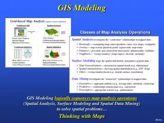
Spatial Statistics • Surface modelingmaps the spatial distribution and pattern of point data… • Map Generalization— characterizes spatial trends (e.g., titled plane) • Spatial Interpolation— deriving spatial distributions (e.g., IDW, Krig) • Other— roving window/facets (e.g., density surface; tessellation) • Data Mininginvestigates the “numerical” relationships in mapped data… • Descriptive— aggregate statistics (e.g., average/stdev, similarity, clustering) • Predictive— relationships among maps (e.g., regression) • Prescriptive— appropriate actions (e.g., optimization) Grid-Based Map Analysis • Spatial analysisinvestigates the “contextual” relationships in mapped data… • Reclassify— reassigning map values (position; value; size, shape; contiguity) • Overlay— map overlay (point-by-point; region-wide; map-wide) • Distance— proximity and connectivity (movement; optimal paths; visibility) • Neighbors— ”roving windows” (slope/aspect; diversity; anomaly) (Berry)
Classes of Spatial Analysis Operators …all spatial analysis involves generating new map values (numbers) as a mathematical or statistical function of the values on another map layer(s) (See |MapCalc\CrossReference for a cross reference of MapCalc operations and ESRI Grid/Spatial Analysis and EDAS) (Berry)
Reclassifying Maps (Berry)
Overlaying Maps (Berry)
Evaluating Habitat Suitability • The Hugag is a curious beast with strong preferences for terrain configuration: • Prefers low elevations (severe nose bleeds at higher altitudes) • Prefers gentle slopes (fear of falling over and unable to get up) • Prefers southerly aspects (a place in the sun) Generating maps of animal habitat… Manual Map Overlay (Binary) Ranking Overlay (Binary Sum) Rating Overlay (Rating Average) (digital slide show Hugag2) (Berry)
Conveying Suitability Model Logic(Short Exercise #3) gentle slopes Elevation Slope Slope Preference Bad 1 to 9 Good Reclassify (Times 1) southerly aspects Elevation Aspect Aspect Preference Bad 1 to 9 Good Habitat Rating Bad 1 to 9 Good (1) Reclassify Overlay lower elevations Elevation Elevation Preference Bad 1 to 9 Good (1) Reclassify Habitat Rating 0= No, 1 to 9 Good Overlay Algorithm Calibrate Weight Base Maps Derived Maps Interpreted Maps Combined Map …while Reclassify and Overlay operations aren’t very exciting, they are frequently used Fact Judgment Covertype Water Mask 0= No, 1= Yes Reclassify Constraint Map (Berry)
Extending Model Criteria (Times 10) (1) (1) forests Forests Forest Proximity Forest Preference Bad 1 to 9 Good (10) • Hugags are 10 times more concerned with slope, forest and water criteriathan aspect and elevation water Water Water Proximity Water Preference Bad 1 to 9 Good (10) gentle slopes Elevation Slope Slope Preference Bad 1 to 9 Good southerly aspects Elevation Aspect Aspect Preference Bad 1 to 9 Good Habitat Rating Bad 1 to 9 Good lower elevations Additional criteria can be added… Elevation Elevation Preference Bad 1 to 9 Good • Hugags would prefer to be in/near forested areas • Hugags would prefer to be near water (Berry)
Reclassifying Maps Overlaying Maps Reclassify & Overlay Operations (MapCalc) (Berry)
Reclassify & Overlay Techniques(Full Exercise #3) • Spatial analysis … useMapCalcto implement the following • SIZECovertype FOR Covertype_size • CLUMPCovertype AT 1 Diagonally FOR Covertype_clumps • SIZECovertype_clumps FOR Covertype_clump_size • CONFIGURECovertype_clumps Edges FOR Covertype_clumps_edges • CONFIGURECovertype_clumps Convexity FOR Covertype_clumps_shape • “RENUMBER Slope / Aspect / Elevation FOR S_Pref / A_pref / E_pref” from Hugag_Habitat.scr script • COMPUTES_Pref Times A_Pref Times E_Pref FOR Binary_model • COMPUTES_Pref Plus A_Pref Plus E_Pref FOR Ranking_model • CROSSTABCovertype WITH Water Simply • CALCULATE(Covertype * 10) + Water FOR CW_codes • COMPOSITECovertype WITH Slope Average FOR Covertype_avgSlope • RENUMBERCovertype ASSIGNING 0 TO 2 THRU 3 FOR OpenWater_binary • COMPUTE OpenWater_binary Times Slope FOR OpenWater_slope (Berry)
Establishing Distance and Connectivity (digital slide show DIST2) (Berry)
Spatial Analysis(Short Exercise #4a) Distance Operators— simple/and effective proximity SPREAD Roads TO 100 Simply FOR Road_prox Impedance to Movement Relative Barrier— terrain steepness Absolute Barrier— water wFriction Friction Difficulty Impassable sFriction Effective Proximity to Roads SPREAD Roads TO 100 Simply THRU Friction FOR Road_hikingprox …far from Roads Simple Proximity to Roads (Berry) (Berry)
Distance/Connectivity Techniques(Full Exercise #4a) • Spatial analysis … useMapCalcto implement the following • SPREADHousing TO 20 FOR Housing_simpleprox • SPREADRoads TO 20 FOR Roads_simpleprox • RENUMBERCovertype ASSIGNING 0 TO 1 • ASSIGNING 3 TO 2 ASSIGNING 7 TO 3 • FOR C_friction • SPREADRoads TO 75 THRU C_friction FOR Road_hikingprox • RENUMBERLocations ASSIGNING 0 TO 2 THRU 5 FOR Ranch • SPREADRanch TO 35 Simply FOR Ranch_simpleprox • RENUMBERRoads ASSIGNING 1 TO 1 THRU 43 FOR R_friction • COVERC_friction WITH R_friction FOR CR_friction • SPREADRanch TO 75 THRU CR_friction FOR Ranch_hikingprox • RENUMBERLocations ASSIGNING 0 TO 1 ASSIGNING 0 TO 3 THRU 5 FOR Cabin • STREAMCabin OVER Ranch_hikingprox FOR Path • COMPUTERanch_hikingprox times path FOR Path_hikingprox (Berry)
Generating an Effective Travel-time Buffer a) superimposition of an analysis grid over the area of interest b) “burns” the store location into its corresponding grid cell c) “burns "primary and residential streets are identified d) travel-time buffer derived from the two grid layers (Store and Streets) (Berry)
…creates an Accumulation Surface identifying travel-time to every location considering absolute (streets) and relative (speed) barriers to movement (digital slide show TTime2) Travel-time is computed as aseries of increasing wavesmoving away from a starting location that are constrained by the streets… Travel-Time Waves (Berry)
…increasing distance from a point forms bowl-shaped accumulation surface …steepest downhill path identifies the optimal path– wave front that got there first. …SPREADing from multiple locations identifies catchment areas– locations closest to starting locations …what do you think the ridges represent? Travel-Time Connectivity (Berry)
Simple distance – symmetrical bowl; constant slope Absolute barrier – abrupt pillars; constant slope Relative barrier – gradual humps with changing slope depending on relative impedance friction) …subtracting two accumulation surfaces identifies relative advantage Zero – equidistant Sign – which store has advantage Magnitude – strength of advantage …what would get if you added the two surfaces? Accumulation Surface Analysis …increasing distance from a point forms bowl-shaped accumulation surface (Berry)
Analysis Frame as Primary Key (Column, Row) Raster (cell) Analysis Frame …V to R Conversion plots customers location in the analysis frame (grid) Latitude, Longitude, C, R Vector (point) …can append any GIS derived information (Col,Row) …Append Col, Row, Lat, Lon of cell location to customer records Customer Database (non-spatial) Customer Database (spatial) …GeoCoding plots customers address on the streets map (Berry)
Clipped Buffer– simple proximity for just the land areas Uphill Buffer– simple proximity to the road for just the areas that are uphill from the road; absolute barrier (uphill only– absolutely no downhill steps) Variable-Width Buffers (Simple/uphill proximity) Simple Buffer– “as-the-crow-flies” proximity to the road; no absolute or relative barriers are considered (Berry)
Seen if new tangent exceeds all previous tangents along the line of sight— At <Viewer_heightValue> Thru <Screens_heightMap>) Onto <Target_heightMap> Establishing Visual Connectivity (Viewshed) Radiate – analogous to a searchlight casting its beam light onto the landscape Simply – viewshed Completely – number of “viewers” that see each location Weighted – viewer cell value is added …like SPREAD, RADIATE starts somewhere (starter cell) and moves through geographic space by steps (wave front) assigning a 1 (seen) to locations with tangents larger than the previous ones (Berry)
Visual exposure identifies how many times each map location is seen from a set of viewer locations Calculating Visual Exposure (# Times Seen) (Berry)
A visual exposure map identifies how many times each location is seen from an “extended eyeball” composed of numerous viewer locations (road network) Visual Exposure from Extended Features Simply – viewshed Completely– number of “viewers” that see each location Weighted – viewer cell value is added (Berry)
Different road types are weighted by the relative number of cars per unit of time …the total “number of cars” replaces the “number of times seen” for each grid location Weighted Visual Exposure (Sum of Viewer Weights) Simply – viewshed Completely – number of “viewers” that see each location Weighted – viewer cell value is added (Berry)
Spatial Analysis(Short Exercise #4b) Visual Exposure Operators — viewshed and visual exposure Roads Elevation RADIATE Roads OVER Elevation AT 1 TO 100 Simply FOR Road_viewshed RADIATE Roads OVER Elevation TO 100 AT 1 Completely FOR Road_VExposure RADIATE Road_classes OVER Elevation TO 100 AT 1 Weighted FOR Road_wVExposure # Cars …not seen …seen a lot Road_classes Viewshed from Roads Visual Exposure from Roads (Berry) (Berry)
Weighted visual exposure map for an ongoing visual assessment in a national recreation area— the project developed visual vulnerability maps from the reservoir in the center of the park and a major highway running through the park. In addition, aesthetic maps were generated based on visual exposure to pretty and ugly places in the park Real-World Visual Analysis (Senior Honors Thesis by University of Denver Geography student Chris Martin, 2003) (Berry)
Line-of-Sight Buffer– identifies all land locations (clipped) within 250m that can be seen from the road… 250m “viewshed” of the road Line-of-Sight Exposure– notes the number of time each location in the buffer is seen Line-of-Sight Noise– locations hidden behind a ridge or farther away from a source (road) greatly decrease noise levels. Variable-Width Buffers (Line-of-sight) (Berry)
SLICE Housing_WeightedVE INTO 4 • FOR Housing_VE_Index • SLICE Roads_VExposure INTO 4 • FOR Roads_VE_Index • ANALYZE Housing_VE_Index • WITH Roads_VE_Index Mean • FOR RH_VE_Index_avg Visual Analysis Techniques(Full Exercise #4b) • Spatial analysis … use MapCalcto implement the following • RADIATE Ranch OVER ELEVATION TO 35 • AT 5 SIMPLY FOR Ranch_viewshed • RADIATE Roads OVER ELEVATION TO 35 • AT 5 SIMPLY FOR Roads_viewshed • RADIATE Roads OVER ELEVATION TO 35 • AT 5 COMPLETELY FOR Roads_VExposure • RADIATE Housing OVER ELEVATION TO 35 • WEIGHTED FOR housing_WeightedVE (Berry)
Characterizing Neighborhoods (Berry)
Min= 0.00 Max= 65.00 Avg= 24.38 Min= 0.00 Max= 64.63 Avg= 26.45 Min= 0.00 Max= 17.25 Avg= 3.56 Min= 0.00 Max= 40.24 Avg= 15.13 Characterizing Terrain Steepness (Slope) Slope is can be calculated several ways– by calculating the best fitting plane to all nine elevation values, or by selecting the maximum, minimum or average of the eight individual slopes (Berry)
Creating a Housing Density Map (Scan Total) The TOTAL number of houses within 500 meters is calculated for each map location (Berry)
Creating a Cover Type Diversity Map (Scan Diversity) …a DIVERSITY map indicates the number of different map values that occur within a window… e.g., cover types. As the window is enlarged, the diversity increases. (Berry)
Spatial Analysis(Short Exercise #5) SCAN Houses Total 0.0 WITHIN 6 CIRCLE FOR Housing_density Most diverse Highest density Houses Housing_density SCAN Covertype Diversity WITHIN 4 CIRCLE FOR Covertype_diversity Covertype Covertype_diversity Most rough SCAN Slopemap CoffVar WITHIN 2 CIRCLE FOR Roughness Slopemap Terrain_roughness Neighbor Operators — summarizing nearby values (Berry) (Berry)
2 Very Edgy 8 Not Edgy Characterizing “Edginess” A simple EDGINESS model for the meadow involves assigning 1 to the meadow (Renumber) and then calculating the total values within a 3x3 window for just the meadow area (Around) (Berry)
Landscape Analysis (Berry)
Neighbor Techniques (Full Exercise #5) • Spatial analysis … use MapCalcto implement the following • SCANCovertype DIVERSITY WITHIN 2 • FOR Covertype_diversity2 • SCANCovertype DIVERSITY WITHIN 4 • FOR Covertype_diversity4 • SCANCOVERTYPE DIVERSITY WITHIN 4 • AROUND ROADS FOR Covertype_diversity4_roads • SCANELEVATION AVERAGE WITHIN 4 FOR Elevation_smooth4 • COMPUTEELEVATION MINUS Elevation_smooth4 FOR Convex_concave_terrain • SCANSLOPE COFFVAR WITHIN 1 FOR Slope_roughness • SLOPESLOPE FOR What? • RENUMBERRanch_hikingprox ASSIGNING PMAP_NULL TO 100 FOR Ranch_hikingprox_mask • SLOPE Ranch_hikingprox_masked FOR What_else? • ORIENTRanch_hikingprox_masked FOR You_have_to_be_kiding! (Berry)
…but before we leave Spatial Analysis (operations for reclassify, overlay, distance and neighbors) to tackle Spatial Statistics, any… Questions? Questions? (Berry)