Download
1 / 45
450 likes | 465 Views
Spatial Filtering. output image. Spatial Filtering Methods (or Mask Processing Methods). Spatial Filtering. The word “filtering” has been borrowed from the frequency domain. Filters are classified as: Low-pass (i.e., preserve low frequencies) High-pass (i.e., preserve high frequencies)

E N D
output image Spatial Filtering Methods (or Mask Processing Methods)
Spatial Filtering • The word “filtering” has been borrowed from the frequency domain. • Filters are classified as: • Low-pass (i.e., preserve low frequencies) • High-pass (i.e., preserve high frequencies) • Band-pass (i.e., preserve frequencies within a band) • Band-reject (i.e., reject frequencies within a band)
output image Spatial Filtering (cont’d) • Spatial filtering is defined by: (1) A neighborhood (2) An operation that is performed on the pixels inside the neighborhood
Spatial Filtering - Neighborhood • Typically, the neighborhood is rectangular and its size • is much smaller than that of f(x,y) • - e.g., 3x3 or 5x5
Spatial filtering - Operation Assume the origin of the mask is the center of the mask. for a 3 x 3 mask: for a K x K mask:
output image Spatial filtering - Operation • A filtered image is generated as the center of the mask moves to every pixel in the input image.
Handling Pixels Close to Boundaries pad with zeroes 0 0 0 ……………………….0 or 0 0 0 ……………………….0
Linear vs Non-LinearSpatial Filtering Methods • A filtering method is linear when the output is a weighted sum of the input pixels. • Methods that do not satisfy the above property are called non-linear. • e.g.,
Linear Spatial Filtering Methods • Two main linear spatial filtering methods: • Correlation • Convolution
w(i,j) Output Image f(i,j) Correlation g(i,j)
Correlation (cont’d) Often used in applications where we need to measure the similarity between images or parts of images (e.g., pattern matching).
Convolution • Similar to correlation except that the mask is first flipped both horizontally and vertically. Note: if w(x,y) is symmetric, that is w(x,y)=w(-x,-y), then convolution is equivalent to correlation!
Example Correlation: Convolution:
2nd derivative of Gaussian 1st derivative of Gaussian Gaussian How do we choose the elements of a mask? • Typically, by sampling certain functions.
Gaussian Filters • Smoothing (i.e., low-pass filters) • Reduce noise and eliminate small details. • The elements of the mask must be positive. • Sum of mask elements is 1 (after normalization)
2nd derivative of Gaussian 1st derivative of Gaussian Filters (cont’d) • Sharpening (i.e., high-pass filters) • Highlight fine detail or enhance detail that has been blurred. • The elements of the mask contain both positive and negative weights. • Sum of the mask weights is 0 (after normalization)
Smoothing Filters: Averaging (cont’d) • Mask size determines the degree of smoothing and loss of detail. original 3x3 5x5 7x7 15x15 25x25
Smoothing Filters: Averaging (cont’d) Example: extract, largest, brightest objects 15 x 15 averaging image thresholding
Smoothing filters: Gaussian • The weights are samples of the Gaussian function σ = 1.4 mask size is a function of σ :
Smoothing filters: Gaussian (cont’d) • σ controls the amount of smoothing • As σ increases, more samples must be obtained to represent • the Gaussian function accurately. σ = 3
Averaging vs Gaussian Smoothing Averaging Gaussian
Smoothing Filters: Median Filtering(non-linear) • Very effective for removing “salt and pepper” noise (i.e., random occurrences of black and white pixels). median filtering averaging
Smoothing Filters: Median Filtering (cont’d) • Replace each pixel by the median in a neighborhood around the pixel.
Sharpening Filters (High Pass filtering) • Useful for emphasizing transitions in image intensity (e.g., edges).
Sharpening Filters (cont’d) • Note that the response of high-pass filtering might be negative. • Values must be re-mapped to [0, 255] sharpened images original image
Sharpening Filters: Unsharp Masking • Obtain a sharp image by subtracting a lowpass filtered (i.e., smoothed) image from the original image: - =
Sharpening Filters: High Boost • Image sharpening emphasizes edges but details (i.e., low frequency components) might be lost. • High boost filter: amplify input image, then subtract a lowpass image. (A-1) + =
Sharpening Filters: High Boost (cont’d) • If A=1, we get a high pass filter • If A>1, part of the original image is added back to the high pass filtered image.
Sharpening Filters: High Boost (cont’d) A=1.9 A=1.4
Sharpening Filters: Derivatives • Taking the derivative of an image results in sharpening the image. • The derivative of an image can be computed using the gradient.
Sharpening Filters: Derivatives (cont’d) • The gradient is a vector which has magnitude and direction: or (approximation)
Sharpening Filters: Derivatives (cont’d) • Magnitude: provides information about edge strength. • Direction: perpendicular to the direction of the edge.
sensitive to vertical edges Δx sensitive to horizontal edges Sharpening Filters: Gradient Computation • Approximate gradient using finite differences:
Sharpening Filters: Gradient Computation (cont’d) • We can implement and using masks: (x+1/2,y) good approximation at (x+1/2,y) (x,y+1/2) * * good approximation at (x,y+1/2) • Example: approximate gradient at z5
Sharpening Filters: Gradient Computation (cont’d) • A different approximation of the gradient: good approximation (x+1/2,y+1/2) * • We can implement and using the following masks:
Sharpening Filters: Gradient Computation (cont’d) • Example: approximate gradient at z5 (ROBERT CROSS) • Other approximations Sobel
Sharpening Filters: Laplacian The Laplacian (2nd derivative) is defined as: (dot product) Approximate derivatives:
Sharpening Filters: Laplacian (cont’d) Laplacian Mask detect zero-crossings
Sharpening Filters: Laplacian (cont’d) Sobel Laplacian