Download
1 / 82
900 likes | 1.3k Views
Explore intensity transformations & spatial filtering techniques in digital image processing. Learn how to enhance images using diverse functions and spatial filters in the spatial domain.

E N D
Chapter 3 Intensity Transformations and Spatial Filtering The images used here are provided by the authors. Objectives: We will learn about different transformations, some seen as enhancement techniques.
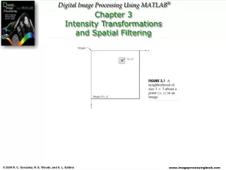
Chapter 3 Intensity Transformations and Spatial Filtering 3.1 Background 3.2 Intensity Transformation Functions 3.2.1 Function imadjust 3.2.2 Logarithmic and Contrast-Stretching Transformations 3.2.3 Some Utility M-Functions for Intensity Transformations 3.3 Histogram Processing and Function Plotting 3.3.1 Generating and Plotting Image Histograms 3.3.2 Histogram Equalization 3.3.3 Histogram Matching (Specification)
3.4 Spatial Filtering 3.4.1 Linear Spatial Filtering 3.4.2 Nonlinear Spatial Filtering 3.5 Image Processing Toolbox Standard Spatial Filters 3.5.1 Linear Spatial Filters 3.5.2 Nonlinear Spatial Filters Summary
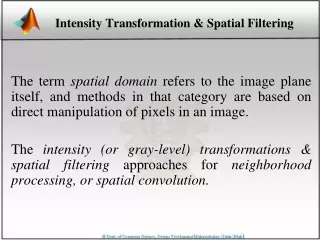
Chapter 3 Intensity Transformations and Spatial Filtering The term spatial domain refers to the image plane itself, and methods in this category are based on direct manipulation of pixels in an image. There are two main important categories of spatial domain processing: 1) intensity (gray level) transformation and spatial filtering. In general the spatial processing is denoted as: g(x,y) = T[f(x,y)], where f(x,y) is the input image, g(x,y) is the output (processed) image, and T is an operator on f defined over a specific neighborhood about point (x,y).
Chapter 3 Intensity Transformations and Spatial Filtering
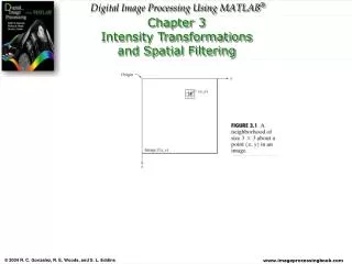
Chapter 3 Intensity Transformations and Spatial Filtering The principal approach for defining spatial neighborhoods about a point (x,y) is to use a square or rectangular region centered at (x,y). This is shown on Figure 3.1 The idea is to move the center of this region pixel to pixel starting at one corner and continue with this procedure until the entire image is covered.
Chapter 3 Intensity Transformations Functions The simplest form of the transform function T is when the neighborhood square is of size 1 x 1 (a single pixel). In this case, the value of g at (x,y) depends only on the intensity of f that pixel and T becomes an intensity or gray-level transformation function. Since only intensity values play a role not (x,y), the transformation function might be written as: s = T(r) where r denotes the intensity of f and s the intensity of g, both at any corresponding point (x,y) in the image.
Example: Consider the following matrix that represent the image data for a 4X4 image. Apply a 2X2 average transformation. I.e. a pixel will be represented by the average of 4 pixels around it. Start from top left. 2 4 10 4 2 16 14 4 4 6 8 2 4 0 2 2
Chapter 3 Intensity Transformations Functions The imadjust function is the basic IPT tool for intensity transformations of gray scale images. g = imadjust(f, [low_in high_in], [low_out high_out], gamma) The above command will map the intensity values in image f to new values in g such that values between low_in and high_in map to values between low_out and high_out.
g = imadjust(f, [low_in high_out], [low_out high_out], gamma) • Notes on imadjust: • Using ([ ]) for low_in, high_in, low_out, and high_out results in the default values [0 1]. • If high value is lower than low value, then the intensity is reversed. • The input image can be of class unit8, unit16, or double and the output image has the same class as the input. • Parameter gamma specifies the shape of the curve that maps the intensity values f to create g. • If gamma is less than 1, the mapping is weighted toward higher (brighter) output.
This is a bit confusing. Let’s go through an example hoping to clear things up. >> f = uint8([0 100 156 222 255 12]) 0 100 156 222 255 12 Which means this values are in the unit8 class, i.e. numbers between 0 to 255. I will use: >> g = imadjust(f, [0.0; 0.2], [0.5 1],1) Which means (this is the tricky part): Map the values between 0 to 0.2*255 i.e. [0 to 51] to values from 0.5*255 = 128 and 255, i.e [128 255], results: 128 255 255 255 255 158
Repeat the same example: >> f = uint8([0 100 156 222 255 12]) 0 100 156 222 255 12 But, this timeI will use: >> g = imadjust(f, [0.2; 0.5], [0.5 1],1) This maps the values between 0.2*255 to 0.5*255: i.e. [51, 128] to values from 0.5*255 = 128 and 255, i.e [128 255], results: 128 209 255 255 255 128
Practice: Suppose: >> f = uint8([0 100 156 222 255 12]) What would you get for: >> g = imadjust(f, [0.4; 0.5], [0.5 1],1) 128 128 255 255 255 128 What would you get for: >> g = imadjust(f, [0.4; 0.5], [1 0.5],1) 255 255 128 128 128 255
Practice: Suppose: >> f = uint8([0 100 156 222 255 12]) What would you get for: >> g = imadjust(f, [0.4; 0.5], [0.5 1],2) 128 128 255 255 255 128 What would you get for: >> g = imadjust(f, [0.4; 0.5], [1 0.5],.2) 255 255 128 128 128 255
a) Digital mammogram • b) Negative image • (f, [0 1] , [1,0]) • c) Adjusted with: • (f, [0.5 0.75] , [0,1]) • d) Enhanced image: • gamma = 2 a b c d
Logarithmic and Contrast-Stretching Transformations Use widely for dynamic range manipulation. Logarithmic transformation is implemented using: g = c*log(1 + double(f) ) where c is a constant. What kind of behavior does this model show?
Logarithmic and Contrast-Stretching Transformations Compresses dynamic range, what does this mean?
Logarithmic Transformations When performing a logarithmic transformation, it is often desirable to bring the resulting compressed values back to the full range of the display. In MATLAB, for 8 bits, we can use: >> gs = im2unit8(mat2gray(g)); Use of mat2gray brings the values to the range [0, 1], and im2unit8 brings them to the range [0, 255].
Example: >> c = 2; >> g = c*log(1 + double(img)) g = 1.3863 6.3561 10.7226 11.0825 5.1299 8.7389 11.0904 8.9547 8.3793 10.7226 7.5684 6.1821 9.4548 11.0825 2.7726 4.1589
>> g1 = mat2gray(g) g1 = 0 0.5121 0.9621 0.9992 0.3858 0.7577 1.0000 0.7799 0.7206 0.9621 0.6371 0.4942 0.8315 0.9992 0.1429 0.2857 >> gs = im2uint8(g1) gs = 0 131 245 255 98 193 255 199 184 245 162 126 212 255 36 73 Original
Fourier Spectrum Same image after a logarithmic transformation
Contrast-Stretching Transformations It compresses the input levels lower than m into a narrow range of dark levels in the output image, and compresses the values above m into a narrow band of light levels in the output. Limiting case: Thresholding
Contrast-Stretching Transformations The function corresponding to the diagram on the left is: Where r represents the intensities of the input image, s denotes the intensity in the output image, and E controls the slope of the function. In MATLAB, this can be written as: g = 1./(1 + (m./(double(f) + eps)).^E)
Original: >> g = 1./(1 + (127./(double(img) + eps)).^2) g = 0.0001 0.0318 0.7359 0.8000 0.0088 0.2739 0.8013 0.3194 0.2076 0.7359 0.1028 0.0266 0.4375 0.8000 0.0006 0.0030
>> g1 = mat2gray(g) g1 = 0 0.0396 0.9184 0.9984 0.0110 0.3418 1.0000 0.3986 0.2590 0.9184 0.1283 0.0331 0.5460 0.9984 0.0006 0.0037 >> gs = im2uint8(g1) gs = 0 10 234 255 3 87 255 102 66 234 33 8 139 255 0 1 Original
Histogram Processing and Function Plotting Plots and histograms of the image date can be used in enhancement of images. A histogram of a digital image with L total possible intensity levels in the range of [0, G] is defined as the discrete function: h(rk) = nk Where rkis the kth intensity level in the interval [0, G] and nk is the number of pixels in the image whose intensity level is rk. The value of G depends on the data class type. For uni8, it is 255, for unit16 it is 65536, and so on. Note that G = L – 1 for images of class unit8 and unit16.
Histogram Processing and Function Plotting Often, it is useful to work with the normalized histograms which is obtained simply by dividing all elements of h(rk) by the total number of pixels in the image: For k = 1, 2, 3, …, L. From basic probability, we know that p(rk) is an estimate of the probability of occurrence of intensity level rk. In MATLAB, the core function too compute image histogram is: h = imhist(f, b) Where f is the input image, h is its histogram, h(rk) and b is the number of bins used in formatting the histogram.
The normalized histogram can be obtained using: h = imhist(f, b)./numel(f) Where numel(f) will give the number of elements in array f. There are several different ways to plot a histogram. The most common one is the bar graph. bar(horz, v, width) Where v is a row vector containing the points to be plotted, horz is a vector of the same dimension as v that contains the increments of the horizontal scale, and width is a number between 0 to 1.
Example: f = uint8([2 30 255 40 20 70 80 80 90 200 30 255 255 60 50 70 255 2 3 40]) h = imhist(f, 20); Produces: h = 3 1 2 2 2 2 2 1 0 0 0 0 0 0 0 1 0 0 0 4 What does this mean? Width = 255 – 2 = 253 Number of bins = 20 Delta = 253/20 = 12.65 Numbers are between: 2 2+12.65 2+2*12.65 2+3*12.65 … 2+20*12.65
What does this mean? >> h1 = (1:20) >> bar(h1, f) f = uint8([2 30 255 40 20 70 80 80 90 200 30 255 255 60 50 70 255 2 3 40]) intensity Bins corresponding to f
Histogram Equalization Assuming pr(rj) where j = 1, 2, …, L denotes the probability of observing an intensity j in an image with n pixels. In general, the histogram of the processed image will not be uniform. In order to make a create a more uniform distribution, we use a histogram equalization which is based on the CDF. The Cumulative Distribution Function (CDF) can be written as:
Histogram Equalization The equalization transformation is defined as: For k = 1, 2, …, L, where skis the intensity value in the output (processed) image corresponding to value rkin the input image.
Example: f = [2 2 4 5 2 5 4 5 2 3 1 6] • r p(x) • 1/12 • 4/12 • 1/12 • 2/12 • 3/12 • 1/12
Cum prob. • rk sk • 1/12 • 5/12 • 6/12 • 8/12 • 11/12 • 12/12
Hist_eq = histeq(r, 15) • Example of Histogram Equalization pdist*255 • r prob cum prob Hist eq • 0 • 1 0.125 0.125 0 • 3 51 • 3 51 • 3 0.1875 0.3125 51 • 4 85 • 4 0.125 0.4375 85 • 5 119 • 5 0.125 0.5625 119 • 6 0.0625 0.625 153 • 9 170 • 9 0.125 0.75 170 • 11 221 • 11 221 • 11 0.1875 0.9375 221 • 12 0.0625 1.0 255 p dist 0 1/15=0.066667 2/15=0.133333 3/15=0.2 4/15=0.266667 5/15=0.333333 6/15=0.4 7/15=0.466667 8/15=0.533333 9/15=0.6 10/15=0.666667 11/15=0.733333 12/15=0.8 13/15=0.866667 14/15=0.933333 15/15=1
Histogram Matching Histogram equalization can achieve enhancement by spreading the levels. However, since the transformation function is based on the histogram of the image it does not change unless the histogram of the image changes. The result is not always successful. Sometimes, we wish the histogram of the image to look like a given histogram. The method used to make the histogram of processed image looks like a given histogram is called histogram matching or histogram specification.
The input levels have probability density function pr(r) and The output levels have the specified probability density function pz(z)
From histogram equalization, we learned that: Results in intensity levels, s, have a uniform probability density functions ps(s). Suppose now we define a variable z with the property H(z): We are trying to find an image with intensity levels z, which have specified density pz(z), from these two equations, we have: Z = H-1(s) = H-1[T(r)] We can find T(r) from the input image. Then we need to find the transformed level z whose PDF is the specified pz(z), as long as we can find H-1. MATLAB: g = histeq(f, hspec) where f is input, hspec is the given histogram.
Spatial Filtering • The neighborhood processing consists of: • Defining a center point, (x,y); • Performing an operation that involves only pixels in a predefined neighborhood about that center point; • Letting the result of that operation be the “response” of the process at that point; • Repeating the process for every point in the image. • The two principal terms used to identify this operation are neighborhood processing and spatial filtering, with the second term being more prevalent. • If the operation is linear, then it is called linear spatial filtering (spatial convolution), otherwise, it is called nonlinear spatial filtering.
Linear Spatial Filtering (LSF) This filtering has its root in the use of the Fourier transform for signal processing in the frequency domain. The idea is to multiply each pixel in the neighborhood by a corresponding coefficient and summing the results to obtain the response at each point (x,y). If the neighborhood is of size m-by-n, then mn coefficients are required. These coefficients are arranged as a matrix called a filter, mask, filter mask, kernel, template, or window. The first three terms are most prevalent. It is not required but is more intuitive to use odd-size masks because they have one unique center point.
There are two closely related concepts in LSF: 1) correlation, 2) convolution Correlation is the process of passing the mask w by the image array f. Mechanically, convolution is the same process, except that w is rotated by 180o prior to passing it by f. In both cases we will compute the sum of products of participating values and will place it at the desired position.
Correlation 0 0 0 1 0 0 0 0 w 1 2 3 2 0 Original f Step 0 0 0 0 1 0 0 0 0 1 2 3 2 0 Zero padding 0 0 0 0 0 0 0 1 0 0 0 0 1 2 3 2 0 0 0 0 0 0 0 0 1 0 0 0 0 0 0 0 0 Zero padding 1 2 3 2 0
Correlation-cont. 0 0 0 0 0 0 0 1 0 0 0 0 0 0 0 0 After Shift 1 1 2 3 2 0 After Shift 4 0 0 0 0 0 0 0 1 0 0 0 0 0 0 0 0 1 2 3 2 0 Last Shift 0 0 0 0 0 0 0 1 0 0 0 0 0 0 0 0 1 2 3 2 0 ‘full’ correlation result 0 0 0 02 3 2 1 0 0 0 0 ‘same’ correlation result 0 02 3 2 1 0 0 0 0
Convolution 0 0 0 1 0 0 0 0 w 0 2 3 2 1 Original f Step 0 0 0 0 1 0 0 0 0 0 2 3 2 1 Zero padding 0 0 0 0 0 0 0 1 0 0 0 0 0 2 3 2 1 0 0 0 0 0 0 0 1 0 0 0 0 0 0 0 0 Zero padding 0 2 3 2 1
Convolution-cont. 0 0 0 0 0 0 0 1 0 0 0 0 0 0 0 0 After Shift 1 0 2 3 2 1 After Shift 4 0 0 0 0 0 0 0 1 0 0 0 0 0 0 0 0 0 2 3 2 1 Last Shift 0 0 0 0 0 0 0 1 0 0 0 0 0 0 0 0 0 2 3 2 1 ‘full’ convolution result 0 0 0 1 2 3 2 0 0 0 0 0 ‘same’ convolution result 0 1 2 3 2 0 0 0