Spatial Filtering

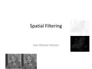
Spatial Filtering Dan Witzner Hansen

Recap • Exercises??? • Feedback • Last lectures?

Digital images • In computer vision we operate on digital (discrete) images: • Sample the 2D space on a regular grid • Quantize each sample (round to nearest integer) • Image thus represented as a matrix of integer values. 2D 1D Adapted from S. Seitz

What is point processing? • Only one pixel in the input has an effect on the output • For example: • Changing the brightness, thresholding, histogram stretching Input Output

Image neighborhoods • Q: What happens if we reshuffle all pixels within the images? • A: Its histogram won’t change. Point-wise processing unaffected. • Need to measure properties relative to small neighborhoods of pixels

Why use proximity • Noise reduction • Smoothing • Feature detection • Correlation

What are they good for? • Improve Search • Search over translations • Classic coarse-to-fine strategy • Search over scale • Template matching • E.g. find a face at different scales • Precomputation • Need to access image at different blur levels • Useful for texture mapping at different resolutions (called mip-mapping) • Image Processing • Editing frequency bands separately • E.g. image blending…

Motivation: noise reduction

Common types of noise • Salt and pepper noise: random occurrences of black and white pixels • Impulse noise: random occurrences of white pixels • Gaussian (additive) noise: variations in intensity drawn from a Gaussian normal distribution Source: S. Seitz

Gaussian noise Ideal Image Noise process >> noise = randn(size(im)).*sigma; >> output = im + noise; Fig: M. Hebert

Changing Sigma and zero mean

First attempt at a solution Replace each pixel with an average of all the values in its neighborhood Assumptions: • Expect pixels to be like their neighbors • Expect noise processes to be independent from pixel to pixel

First attempt at a solution • Let’s replace each pixel with an average of all the values in its neighborhood • Moving average in 1D: Source: S. Marschner

Weighted Moving Average • Can add weights to our moving average • Weights [1, 1, 1, 1, 1] / 5 Source: S. Marschner

Weighted Moving Average • Non-uniform weights [1, 4, 6, 4, 1] / 16 Source: S. Marschner

Neighborhood processing Several pixels in the input has an effect on the output Input Output

Moving Average In 2D Source: S. Seitz

Correlation filtering Say the averaging window size is 2k+1 x 2k+1: Attribute uniform weight to each pixel Loop over all pixels in neighborhood around image pixel F[i,j] Now generalize to allow different weights depending on neighboring pixel’s relative position: Non-uniform weights

Correlation filtering This is called cross-correlation, denoted Filtering an image: replace each pixel with a linear combination of its neighbors. The filter “kernel” or “mask” H[u,v] is the prescription for the weights in the linear combination. Assume the kernel H has weights 0 ‘outside’ the finite region

1 1 1 1 1 1 1 1 1 Averaging filter What values belong in the kernel H for the moving average example? ? “box filter”

Smoothing by averaging depicts box filter: white = high value, black = low value filtered original

Gaussian filter What if we want nearest neighboring pixels to have the most influence on the output? This kernel is an approximation of a Gaussian function: Source: S. Seitz

Smoothing with a Gaussian

Gaussian filters What parameters matter here? Size of kernel or mask • Note, Gaussian function has infinite support, but discrete filters use finite kernels σ = 5 with 10 x 10 kernel σ = 5 with 30 x 30 kernel

Gaussian filters Variance of Gaussian: determines extent of smoothing σ = 2 with 30 x 30 kernel σ = 5 with 30 x 30 kernel

Matlab >> hsize = 10; >> sigma = 5; >> h = fspecial(‘gaussian’ hsize, sigma); >> mesh(h); >> imagesc(h); >> outim = imfilter(im, h); >> imshow(outim);

The effect of smoothing and noise Wider smoothing kernel  More noise 

Boundary issues • What is the size of the output? • MATLAB: filter2(g, f, shape) / conv2 • shape = ‘full’: output size is sum of sizes of f and g • shape = ‘same’: output size is same as f • shape = ‘valid’: output size is the difference of sizes of f and g full same valid g g g g f f g f g g g g g Source: S. Lazebnik g g

Boundary issues • What about near the edge? • the filter window falls off the boundaries of the image • methods: clip filter (black) wrap around copy edge reflect across edge Source: S. Marschner

Boundary issues in Matlab clip filter (black): imfilter(f, g, 0) wrap around:imfilter(f, g, ‘circular’) copy edge: imfilter(f, g, ‘replicate’) reflect across edge: imfilter(f, g, ‘symmetric’) Source: S. Marschner

Filtering an impulse signal What is the result of filtering the impulse signal (image) F with the arbitrary kernel H? ?

Convolution • Convolution: • Flip the filter in both dimensions (bottom to top, right to left) • Then apply correlation F H Notation for convolution operator

Convolution vs. correlation Convolution Cross-correlation

Shift invariant linear system • Shift invariant: Operator behaves the same everywhere, i.e. the value of the output depends on the pattern in the image neighborhood, not the position of the neighborhood. • Linear: Superposition: h * (f1 + f2) = (h * f1) + (h * f2) Scaling: h * (kf) = k (h * f)

Properties of convolution • Linear & shift invariant • Commutative: f* g = g * f • Associative (f * g) * h = f * (g * h) • Identity: unit impulse e = […, 0, 0, 1, 0, 0, …]. f* e = f • Differentiation:

How to do color blurring?

1 0 0 0 0 1 0 0 0 0 0 1 1 0 0 0 2 0 1 1 0 0 1 1 0 0 1 0 1 0 0 0 0 0 0 1 Predict the filtered outputs = ? = ? * * - = ? *

0 0 0 0 1 0 0 0 0 Practice with linear filters ? Original Source: D. Lowe

0 0 0 0 1 0 0 0 0 Practice with linear filters Original Filtered (no change) Source: D. Lowe

0 0 0 0 0 1 0 0 0 Practice with linear filters Original Shifted left by 1 pixel with correlation Source: D. Lowe

1 1 1 1 1 1 1 1 1 Practice with linear filters Original Blur (with a box filter) Source: D. Lowe

0 1 0 1 1 0 1 0 1 2 1 0 1 0 1 0 1 0 Practice with linear filters - ? Original Source: D. Lowe

0 1 0 1 1 0 1 0 1 2 1 0 1 0 1 0 1 0 Practice with linear filters - Original • Sharpening filter • Accentuates differences with local average Source: D. Lowe

Spatial Filtering