Download

1 / 64
640 likes | 646 Views
CHAPTER 35 Population Dynamics. Modules 35.1 – 35.5. Keep track of all graphing exericises!!! If you are not sure how to get data, ask!!!!. The Spread of Shakespeare's Starlings.

E N D
CHAPTER 35Population Dynamics Modules 35.1 – 35.5
Keep track of all graphing exericises!!! If you are not sure how to get data, ask!!!!
The Spread of Shakespeare's Starlings • In the 1800s and early 1900s, introducing foreign species of animals and plants to North America was a popular, unregulated activity • In 1890, a group of Shakespeare enthusiasts released about 120 starlings in New York's Central Park • It was part of a project to bring to America every bird species mentioned in Shakespeare’s works
Their population is estimated at well over 100 million Current • Today, the starling range extends from Mexico to Alaska 1955 Current 1955 1945 1935 1925 1945 1905 1915 1925 1935 1925 1935
Starlings are omnivorous, aggressive, and tenacious • They cause destruction and often replace native bird species • Attempts to eradicate starlings have been unsuccessful • Over 5 million starlings have been counted in a single roost
The starling population in North America has some features in common with the global human population • Both are expanding and are virtually uncontrolled • Both are harming other species • Population ecology is concerned with changes in population size and the factors that regulate populations over time
35.1 Populations are defined in several ways • Ecologists define a population as a single-species group of individuals that use common resources and are regulated by the same environmental factors • Individuals in a population have a high likelihood of interacting and breeding with one another • Researchers must define a population by geographic boundaries appropriate to the questions being asked • Small contained area, i.e. sea anemones in a tide pool • Expanded view, i.e. humans exposed to HIV includes all humans on planet. • Two important characteristics of population included density and dispersion.
POPULATION STRUCTURE AND DYNAMICS 35.2 Density and dispersion patterns are important population variables • Population density is the number of individuals in a given area or volume • It is sometimes possible to count all the individuals in a population • More often, density is estimated by sampling • Divide area in plots, count numbers in a few of those plots, and get an average density, then multiply average times total number of plots.
One useful sampling technique for estimating population density is the mark-recapture method – see Eco packet exercise Figure 35.2A
The dispersion pattern of a population refers to the way individuals are spaced within their area • Clumped • Uniform • Random
This is the most common dispersion pattern in nature • It often results from an unequal distribution of resources in the environment • Clumped dispersion is a pattern in which individuals are aggregated in patches Figure 35.2B
A uniform pattern of dispersion often results from interactions among individuals of a population • Territorial behavior and competition for water are examples of such interactions Figure 35.2C
Random dispersion is characterized by individuals in a population spaced in a patternless, unpredictable way • Example: clams living in a mudflat • Environmental conditions and social interactions make random dispersion rare
35.3 Idealized models help us understand population growth • Idealized models describe two kinds of population growth • exponential growth • logistic growth
Exponential growth is the accelerating increase that occurs during a time when growth is unregulated • A J-shaped growth curve, described by the equation G = rN, is typical of exponential growth • G = the population growth rate • r = the intrinsic rate of increase, or an organism's maximum capacity to reproduce (birth rate – death rate) • N = the population size
Exponential growth model. This models the growth of a population under ideal conditions with unlimited resources. The rate of growth is exponential and depends on the number of individuals in the population: • The graph shows a J-shaped curve, representing population size increasing without limit. As N increases, so does G. This type of growth, if exhibited by a bacterium growing in an unlimited environment, would result in an inconceivably large number of bacteria in less than two days • No population can grow exponentially indefinitley • Starlings 100 -> 1 million in 100 years • 2 elephants -> 19 million in 750 years
Slope = Growth rate Figure 35.3A
It tends to level off at carrying capacity • Carrying capacity is the maximum population size that an environment can support at a particular time with no degradation to the habitat • Logistic growth is slowed by population-limiting factors Figure 35.3B
K = carrying capacity • The term (K - N)/Kaccounts for the leveling off of the curve • K varies based on species and resources available • The equation G = rN(K - N)/Kdescribes a logistic growth curve Figure 35.3C
a population's growth rate will be low when the population size is either small or large (death rate rises/birth rate falls) • a population’s growth rate will be highest when the population is at an intermediate level relative to the carrying capacity (birth rate rises/ death rate falls) • Neither model perfect, represents a starting point. • The logistic growth model predicts that
35.4 Multiple factors may limit population growth • Increasing population density directly influences density-dependent rates • such as declining birth rate or increasing death rate • The regulation of growth in a natural population is determined by several factors • limited food supply • the buildup of toxic wastes • increased disease • predation
Field studies of the song sparrow have demonstrated that birth rates may decline as a limited food supply is divided among more and more individuals Figure 35.4A
Density-independent factors limit population no matter the size and are often abiotic factors, i.e. fires, flood, storms, seasonal temperature change or moisture, and human activity • Aphids show exponential growth in the spring and then rapidly die off when the climate becomes hot and dry in the summer Figure 35.4B
Density-dependent birth and death rates • Abiotic factors such as climate and disturbances • Populations often fluctuate in number • A natural population of song sparrows often grows rapidly and is then drastically reduced by severe winter weather • Most populations are probably regulated by a mixture of factors Figure 35.4C
35.5 Some populations have "boom-and-bust" cycles • Some populations go through boom-and-bust cycles of growth and decline • Example: the population cycles of the lynx and the snowshoe hare • The lynx is one of the main predators of the snowshoe hare in the far northern forests of Canada and Alaska
Lynx and hare • http://www.footprintnetwork.org/en/index.php/GFN/page/personal_footprint/
About every 10 years, both hare and lynx populations have a rapid increase (a "boom") followed by a sharp decline (a "bust") Figure 35.5
For the lynx, prey availability often determines population changes. • Recent studies suggest that the 10-year cycles of the snowshoe hare are largely driven by • Excessive predation. . . • But they are also influenced by fluctuations in the hare's food supply • Population cycles may also result from a time lag in the response of predators to rising prey numbers
LIFE HISTORIES AND THEIR EVOLUTION 35.6 Life tables track mortality and survivorship in populations • Life tables and survivorship curves predict an individual's statistical chance of dying or surviving during each interval in its life • Life tables predict how long, on average, an individual of a given age can expect to live
This table was compiled using 1995 data from the U.S. Centers for Disease Control Table 35.6
Population ecologists have adopted this technique, constructing life tables for various plant and animal species
Three types of survivorship curves reflect important species differences in life history • Survivorship curves plot the proportion of individuals alive at each age Figure 35.6
Survivorship curves • Type 1 (whales, elephants, humans) = low birth rates, low infant mortality, and life histories that fit the K-selection model • Type 2 (squirrels, Hydra) = intermediate • Type 3 (oysters, sea lettuce) = high birth rates, high infant mortality and life histories fitting the r-selection model
35.7 Evolution shapes life histories • An organism's life history is the series of events from birth through reproduction to death • Life history traits include • the age at which reproduction first occurs • the frequency of reproduction • the number of offspring • the amount of parental care given • the energy cost of reproduction
Experimentaltransplant ofguppies • The effects of predation on life history traits of guppies has been tested by field experiments for several years. • Heritability demonstrated by retention of characteristics over generations in predator-free environments. • Guppies from pike-cichlid population moved to where small offspring were preyed on. Soon fewer, larger offspring produced Predator: Killifish;preys mainly onsmall guppies Guppies:Larger atsexual maturitythan those in “pike-cichlid”pools Predator: Pike-cichlid;preys mainly on largeguppies Guppies: Smaller atsexual maturity thanthose in “killifish” pools Figure 35.7A
The agave illustrates what ecologists call "big-bang reproduction" • It is able to store nutrients until environmental conditions favor reproductive success • Might not bloom for years, until large enough rainfall acts as trigger. • In nature, every population has a particular life history adapted to its environment Figure 35.7B
Natural selection favors a combination of life history traits that maximizes an individual's output of viable, fertile offspring
Selection for life history traits that maximize reproductive success in uncrowded, unpredictable environments is called r-selection • Such populations maximize r, the intrinsic rate of increase • Individuals of these populations mature early and produce a large number of offspring at a time • Many insect and weed species exhibit r-selection
Selection for life history traits that maximize reproductive success in populations that live at densities close to the carrying capacity (K) of their environment is called K-selection • Individuals mature and reproduce at a later age and produce a few, well-cared-for offspring • Mammals exhibit K-selection
THE HUMAN POPULATION 35.8 Connection: The human population has been growing exponentially for centuries • The human population as a whole has doubled three times in the last three centuries • The human population now stands at about 6.1 billion and may reach 9.3 billion by the year 2050 • Most of the increase is due to improved health and technology • These have affected death rates
The history of human population growth Figure 35.8A
The ecological footprint represents the amount of productive land needed to support a nation’s resource needs • The ecological capacity of the world may already be smaller than its ecological footprint
Ecological footprint in relation to ecological capacity Figure 35.8B
The exponential growth of the human population is probably the greatest crisis ever faced by life on Earth Figure 35.8C
The case for curing cancer • Is finding a cure for cancer a good thing as related to the overall population problems facing the world today? • Think about it for a few moments and then discuss with your partner pros and cons for curing cancer.
Red Alert!!!! Extra Credit!!!!! 25 pts. !!!!!!! • What’s your ecological footprint? • New website see home page for link and assignment information. • DUE WED May 7th!!!