Download

1 / 25
270 likes | 357 Views
Delve into the world of stochastic models, random functions, and time series analysis. Learn about distribution properties, multivariate normal processes, and the Kolmogorov extension theorem.

E N D
Stochastic models - time series. Random process. an infinite collection of consistent distributions probabilities exist Random function. family of random variables, {Y(t;), t Z, } Z = {0,±1,±2,...}, a sample space
Specified if given F(y1,...,yn;t1 ,...,tn ) = Prob{Y(t1)y1,...,Y(tn )yn } n = 1,2,... F's are symmetric in the sense F(y;t) = F(y;t), a permutation F's are compatible F(y1 ,...,ym ,,...,;t1,...,tm,tm+1,...,tn} = F(y1,...,ym;t1,...,tm) m+1 t = 2,3,...
Finite dimensional distributions First-order F(y;t) = Prob{Y(t) t} Second-order F(y1,y2;t1,t2) = Prob{Y(t1) y1 and Y(t2) y2} and so on
Normal process/series. Finite dimension distributions multivariate normal Multivatiate normal. Entries linear combinations of i.i.d standard normals Y = + Z : s by 1: s by r Y: s by 1Z: Nr(0,I) I: r by r identity E(Y) = var(Y) = ' s by s Conditional marginals linear in Y2 when condition on it
Other methods i) Y(t;), : random variable ii) urn model iii) probability on function space iv) analytic formula Y(t) = cos(t + ) ,: fixed : uniform on (-,]
There may be densities The Y(t) may be discrete, angles, proportions, vectors, ... Kolmogorov extension theorem. To specify a stochastic process give the distribution of any finite subset {Y(1),...,Y(n)} in a consistent way, in A
Moment functions. Mean function cY(t) = E{Y(t)} = y dF(y;t) = y f(y;t) dy if continuous = yjf(yj; t) if discrete E{1Y1(t) + 2Y2(t)} =1c1(t) +2c2(t) vector-valued case Signal plus noise: Y(t) = S(t) + (t) e.g. S(.) fixed, or random
Second-moments. autocovariance function cYY(s,t) = cov{Y(s),Y(t)} = E{Y(s)Y(t)} - E{Y(s)}E{Y(t)} non-negative definite jkcYY(tj , tk ) 0 scalars var {jY(ti)} crosscovariance function c12(s,t) = cov{Y1(s),Y2(t)}
Stationarity. Joint distributions, {Y(t+u1),...,Y(t+uk-1),Y(t)}, do not depend on t for k=2,3,... Often reasonable in practice particularly for some time stretches Replaces "identically distributed" (i.i.d.)
mean E{Y(t)} = cY for t in Z autocovariance function cov{Y(t+u),Y(t)} = cYY(u) t,u in Z u: lag = E{Y(t+u)Y(t)} if mean 0 autocorrelation function(u) = corr{Y(t+u),Y(t)}, |(u)| 1 crosscovariance function cov{X(t+u),Y(t)} = cXY(u)
joint density Prob{x < Y(t+u) < x+dx and y < Y(t) < y+ dy} = f(x,y,u) dxdy
(*) Extend to case of > 2 variables
Some useful modelsbrief switch of notation Purely random / white noise often mean 0 Building block
Random walk not stationary
Moving average, MA(q) From (*) stationary
MA(1) 0=1 1 = -.7 Estimate of (k)
Backward shift operator remember translation operator T Linear process. Need convergence condition, e.g. |i | or |i |2 <
autoregressive process, AR(p) first-order, AR(1) Markov * Linear process invertible For convergence in probability/stationarity
a.c.f. of ar(1) from (*) p.a.c.f. corr{Y(t),Y(t-m)|Y(t-1),...,Y(t-m+1)} linearly = 0 for m p when Y is AR(p)
In general case, Useful for prediction
ARMA(p,q) (B)Xt = (B)Zt
ARIMA(p,d,q). Xt = Xt - Xt-1 2Xt = Xt - 2Xt-1 + Xt-2
Yule-Walker equations for AR(p). Sometimes used for estimation Correlate, with Xt-k, each side of
Cumulants. Extension of mean, variance, covariance cum(Y1 , Y2 , ..., Yk ) useful for nonlinear relationships, approximations, ... multilinear functional 0 if some subset of variantes independent of rest 0 of order > 2 for normal normal is determined by its moments, CLT proof