Download
1 / 11
110 likes | 121 Views
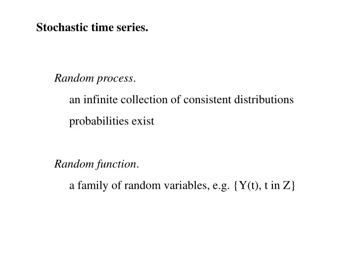
Stochastic time series. Random process . an infinite collection of consistent distributions probabilities exist Random function . a family of random variables, e.g. {Y(t), t in Z}. Specified if given

E N D
Stochastic time series. Random process. an infinite collection of consistent distributions probabilities exist Random function. a family of random variables, e.g. {Y(t), t in Z}
Specified if given F(y1,...,yn;t1 ,...,tn ) = Prob{Y(t1)y1,...,Y(tn )yn } that are symmetric F(y;t) = F(y;t), a permutation compatible F(y1 ,...,ym ,,...,;t1,...,tm,tm+1,...,tn} = F(y1,...,ym;t1,...,tm)
Finite dimensional distributions First-order F(y;t) = Prob{Y(t) t} Second-order F(y1,y2;t1,t2) = Prob{Y(t1) y1 and Y(t2) y2} and so on
Other methods i) Y(t;), : random variable ii) urn model iii) probability on function space iv) analytic formula Y(t) = cos(t + ) : fixed : uniform on (-,]
There may be densities The Y(t) may be discrete, angles, proportions, ... Kolmogorov extension theorem. To specify a stochastic process give the distribution of any finite subset {Y(1),...,Y(n)} in a consistent way, in A
Moment functions. Mean function cY(t) = E{Y(t)} = y dF(y;t) = y f(y;t) dy if continuous = yjf(yj; t) if discrete E{1Y1(t) + 2Y2(t)} =1c1(t) +2c2(t) vector-valued case mean level - signal plus noise: S(t) + (t) S(.): fixed
Second-moments. autocovariance function cYY(s,t) = cov{Y(s),Y(t)} = E{Y(s)Y(t)} - E{Y(s)}E{Y(t)} non-negative definite jkcYY(tj , tk ) 0 scalars crosscovariance function c12(s,t) = cov{Y1(s),Y2(t)}
Stationarity. Joint distributions, {Y(t+u1),...,Y(t+uk-1),Y(t)}, do not depend on t for k=1,2,... Often reasonable in practice - for some time stretches Replaces "identically distributed"
mean E{Y(t)} = cY for t in Z autocovariance function cov{Y(t+u),Y(t)} = cYY(u) t,u in Z u: lag = E{Y(t+u)Y(t)} if mean 0 autocorrelation function(u) = corr{Y(t+u),Y(t)}, |(u)| 1 crosscovariance function cov{X(t+u),Y(t)} = cXY(u)
Higher order moments and cumulants. multilinear functional 0 if some subset of variantes independent of rest 0 of order > 2 for normal normal is determined by its moments
Product moment functions. mY...Y (t1 ,...,tk ) = E{Y(t1 )...Y(tk )} Cumulant functions. cY...Y (t1 ,...,tk ) = cum{Y(t1 ),...,Y(tk )}