TIME SERIES ANALYSIS Time Domain Models : Red Noise; AR and ARMA models

LECTURE 7 TIME SERIES ANALYSIS Time Domain Models: Red Noise; AR and ARMA models Supplementary Readings: Wilks, chapters 8

Recall: Statistical Model [Observed Data] = [Signal] + [Noise] “noise” has to satisfy certain properties! If not, we must iterate on this process... We will seek a general method of specifying just such a model…

Weak Stationarity (Covariance Stationarity) statistics are a function of lag k but not absolute time t • Cyclostationarity statistics are a periodic function of lag k We conventionally assume Stationarity Statistics of the time series don’t change with time • Strict Stationarity

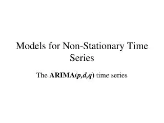
Autoregressive Moving-Average Model(“ARMA”) ARMA(K,M) MODEL Box and Jenkins (1976) Time Series Modeling All linear time series models can be written in the form: We assume that e are Gaussian distributed.

Suppose k=1, and definef1  r Time Series Modeling All linear time series models can be written in the form: Consider Special case of simple Autoregressive AR(k) model (qm=0) Special case of a Markov Process (a process for which the state of system depends on previous states) This should look familiar!

Assume process is zero mean, then Time Series Modeling All linear time series models can be written in the form: Consider Special case of simple Autoregressive AR(k) model (qm=0) Suppose k=1, and definef1  r Lag-one correlated process or “AR(1)” process…

AR(1) Process For simplicity, we assume zero mean

AR(1) Process Let us take this series as a random forcing

AR(1) Process Blue: r=0.4 Red:r=0.7 Let us take this series as a random forcing

AR(1) Process What is the standard deviation of an AR(1) process?

AR(1) Process Blue: r=0.4 Red:r=0.7 Green:r=0.9

Variance is infinite! AR(1) Process Random Walk (“Brownian Motion”) How might we try to turn this into a stationary time series? Supposer=1 Not stationary

AR(1) Process Autocorrelation Function Let us define the lag-k autocorrelation: We can approximate: Let us assume the series x has been de-meaned…

AR(1) Process Autocorrelation Function Let us define the lag-k autocorrelation: Let us define the lag-k autocorrelation: Then:

CO2 since 1976 Autocorrelation Function

AR(1) Process Autocorrelation Function Recursively, we thus have for an AR(1) process, (Theoretical)

r=0.5 N=100 “tcf.m” scf.m “rednoise.m” AR(1) Process Autocorrelation Function

AR(1) Process Autocorrelation Function r=0.5 N=100 r=0.5 N=500 “rednoise.m” “rednoise.m”

AR(1) Process Autocorrelation Function r=0.23 N=1000 Glacial Varves

AR(1) Process Autocorrelation Function r=0.75 N=144 Northern Hem Temp

AR(1) Process Autocorrelation Function r=0.54 N=144 Northern Hem Temp (linearly detrended)

AR(1) Process Autocorrelation Function Dec-Mar Nino3

AR(1) Process The sampling distribution for r is given by the sampling distribution for the slope parameter in linear regression!

AR(1) Process The sampling distribution for r is given by the sampling distribution for the slope parameter in linear regression! How do we determine if r is significantly non-zero? This is just the t test!

AR(1) Process When Serial Correlation is Present, the variance of the mean must be adjusted, Variance inflation factor Recall for AR(1) series, This effects the significance of regression/correlation as we saw previously…

AR(1) Process Supposer 1 This effects the significance of regression/correlation as we saw previously…

Now consider an AR(K) Process For simplicity, we assume zero mean Multiply this equation by xt-k’ and sum,

Use AR(K) Process Yule-Walker Equations

AR(K) Process Yule-Walker Equations Several results obtained for the AR(1) model generalize readily to the AR(K) model:

AR(K) Process Yule-Walker Equations The AR(2) model is particularly important because of the range of behavior it can describe w/ a parsimonious number of parameters The Yule-Walker equations give:

AR(2) Process Which readily gives: The AR(2) model is particularly important because of the range of behavior it can describe w/ a parsimonious number of parameters The Yule-Walker equations give:

For stationarity, we must have: f2 +1 -1 f1 -2 -1 0 1 2 AR(2) Process Which readily gives:

For stationarity, we must have: f2 +1 -1 f1 -2 -1 0 1 2 AR(2) Process Which readily gives: Note that this model allows for independentlag-1 and lag-2 correlation, so that both positive correlation and negative correlation are possible...

For stationarity, we must have: “artwo.m” AR(2) Process Which readily gives: Note that this model allows for independentlag-1 and lag-2 correlation, so that both positive correlation and negative correlation are possible...

Bayesian Information Criterion Akaike Information Criterion AR(K) Process Selection Rules The minima in AIC or BIC represent an ‘optimal’ tradeoff between degrees of freedom and variance explained

Multivariate ENSO Index (“MEI”) AR(K) Process ENSO

AR(1) Fit Autocorrelation Function Dec-Mar Nino3

AR(2) Fit Autocorrelation Function Dec-Mar Nino3 (m>2)

AR(3) Fit Autocorrelation Function Dec-Mar Nino3 Theoretical AR(3) Fit

AR(K) Fit Autocorrelation Function Dec-Mar Nino3 Minimum in BIC? Minimum in AIC? Favors AR(K) Fit for K=?

MA model Now, consider the casefk=0 Pure Moving Average (MA) model, represents a running mean of the past M values. Consider case where M=1…

MA(1) model Now, consider the casefk=0 Consider case where M=1…

ARMA(1,1) model

TIME SERIES ANALYSIS Time Domain Models : Red Noise; AR and ARMA models