Download
1 / 1
40 likes | 297 Views
Hydrologic Model Development and Calibration: The Bi-Objective Approach for Comparing Model Performance. Masoud Asadzadeh, Angela MacLean, Bryan Tolson, Donald Burn Dept. of Civil & Environmental Engineering, University of Waterloo. CG21A-31. ABSTRACT

E N D
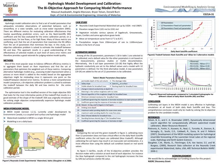
Hydrologic Model Development and Calibration: The Bi-Objective Approach for Comparing Model Performance Masoud Asadzadeh, Angela MacLean, Bryan Tolson, Donald Burn Dept. of Civil & Environmental Engineering, University of Waterloo CG21A-31 ABSTRACT • Hydrologic model calibration aims to find a set of model parameters that adequately simulates observations of watershed behavior, such as streamflow, or a state variable, such as snow water equivalent (SWE). There are different metrics for evaluating calibration effectiveness that involve quantifying prediction errors, such as the Nash-Sutcliffe (NS) coefficient and the bias evaluated for the entire calibration period, on a seasonal basis, for low flows, or for high flows. Many of these metrics are conflicting such that the set of parameters that maximizes the NS differs from the set of parameters that minimizes the bias. In this study, a bi-objective calibration problem is solved to estimate the tradeoff between NS and bias. This approach results in a good understanding of the effectiveness of selected models at each level of every error metric and therefore provides a good rationale for judging relative model quality. • Case Study • Reynolds Creek Experimental Watershed set up by USDA - mid 1960’s • Elevation ranges from 1101 msl to 2241 msl • Vegetation includes various species of Sagebrush, Greasewoods, Aspen, Conifers and some agriculture graze lands • Mean air temperature varies from 4.7˚C to 8.9˚C • Precipitation ranges from 230mm/year of rain to 1100mm/year mostly in the form of snow Alternative Models Among all the 33 parameters, parameters 1-18 in table 1 are selected to be calibrated, and a default value for the other parameters is set based on the measurements, previous studies or CLASS documentation. Alternatively, the 6 soil layer parameters (13-18) that highly affect the hydraulic conductivity are set to the default values and a model with 12 parameters is defined. For the third alternative model, 6 new parameters (19-24) are added to the set of 12 parameters to be calibrated. Figure2) Tradeoff between Nash Sutcliffe and %Bias for 3 alternative models METHODS • One of the most popular ways to balance different efficiency metrics is to aggregate them based on their importance and find the set of parameters that optimizes the weighted sum of these metrics. Comparing alternative hydrologic models (e.g., assessing model improvement when a process or more detail is added to the model) based on the aggregated objectives might be misleading since it represents one point on the tradeoff between desired error metrics. To derive a more comprehensive model comparison, a bi-objective calibration problem is solved to estimate the tradeoff between the daily NS and bias metrics for the entire calibration period. • The optimization tool is the modified version of the single objective DDS that looks for the most informative points of the tradeoff that results in a good estimate of the shape of the tradeoff. DDS was originally introduced for solving single objective computationally expensive hydrologic model calibration problems. • MESH HYDROLOGIC MODEL • MESH model (version 1.2.1), currently under development by Environment Canada, is a coupled land-surface and hydrologic model • Watershed modelled in MESH is a single 30 km grid • Modelling is on a daily basis Table1) Model Parameters Description Figure3) Observed hydrograph compared to 3 simulated hydrographs for different values of daily Nash Sutcliffe (NS) and Bias CONCLUSION Calibrating soil layers in the MESH model is very effective in hydrologic simulations at all levels of both daily Nash Sutcliffe and bias. This comprehensive conclusion could only be made by solving the bi-objective problem for the candidate models. REFERENCES • Tolson, B. A., and C. A. Shoemaker (2007), Dynamically dimensioned search algorithm for computationally efficient watershed model calibration, Water Resources Research. • Pietronio, A., Fortin, V., Kouwen, N., Neal, C., Turcotte, R., Davison, B., Verseghy, D., Soulis, E.D., Caldwell, R., Evora, N. and P. Pellerin (2007), Development of the MESH modeling system for hydrological ensemble forecasting of the Laurentian Great Lakes at the regional scale, Hydrology and Earth System Sciences. • Slaughter, C.W., Marks, D., Flerchinger, G.N, Van Vactor, S.S. and M. Burgess, (2000), Research Data collection at the Reynolds Creek experimental Watershed, Idaho, USA, ARS Technical Bulletin NWRC-2000-2. RESULTS • Comparing the red and the green tradeoffs in figure 2, calibrating more than 12 parameters does not have critical effect on the daily Nash Sutcliffe coefficient unless the soil layers are calibrated (blue tradeoff). Although calibrating the soil layers may result in an inaccurate soil combination, it is more effective than using the default soil condition based on real world values. As figure 3 clarifies, results of the bi-objective problem provides the decision maker with a solution at each level of each objective. For instance the blue hydrograph compared to the red hydrograph increases the bias by 10% but achieves a better NS value. ACKNOWLEDGMENT • We would like to acknowledge our funding source for this project: NSERC Discovery Grant • Figure1) Reynolds Creek Experimental Watershed, Idaho (Slaughter et al.2000)