Download
1 / 79
800 likes | 946 Views
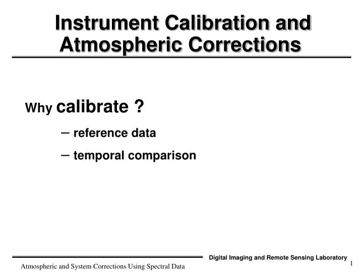
Instrument Calibration and Atmospheric Corrections. Why calibrate ? reference data temporal comparison. ELM. DC. DC or L. R( ). R( ). Band 1 Band 2. Model Based Estimates of R. clouds. DC or L. R predicted by model, e.g. Bio-optical model

E N D
Instrument Calibration and Atmospheric Corrections Why calibrate ? • reference data • temporal comparison Atmospheric and System Corrections Using Spectral Data
ELM DC DC or L R() R() Band 1 Band 2 Atmospheric and System Corrections Using Spectral Data
Model Based Estimates of R clouds DC or L R predicted by model, e.g. Bio-optical model for R() as a function of coloring agents ([C], [CDOM], [TSS]) R() Atmospheric and System Corrections Using Spectral Data
Standard Surfaces Clouds Significant potential for error if only limited samples are available or target, variability is high. DC or L Deep Vegetation R() Band 1 Atmospheric and System Corrections Using Spectral Data
Atmospheric and System Corrections Using Spectral Data (cont’d) • Note ELM can also be used with calibrated system • Pros • removes atmospheric and sensor artifacts • simple and direct if good ground data available Atmospheric and System Corrections Using Spectral Data
Atmospheric and System Corrections Using Spectral Data (cont’d) • cons • requires large known targets • assumes uniform correction across image • can introduce sizeable errors if reference reflectance is not well-known or significantly different than target reflectance Atmospheric and System Corrections Using Spectral Data
Atmospheric and System Corrections Using Spectral Data (cont’d) calibrating sensors • laboratory calibration • spectral calibration • band center • relative spectral response • FW HM • absolute calibration to radiance Atmospheric and System Corrections Using Spectral Data
AVIRIS Airborne Visible/Infrared Imaging Spectrometer (AVIRIS) Figure 3 shows a detail of the AVIRIS onboard calibrator which is used for monitoring and updating the laboratory calibration of AVIRIS. Atmospheric and System Corrections Using Spectral Data
AVIRIS (cont’d) Figure 3. In-flight calibrator configuration Atmospheric and System Corrections Using Spectral Data
AVIRIS (cont’d) Figure 1. a) Laboratory spectral calibration set-up. Atmospheric and System Corrections Using Spectral Data
AVIRIS (cont’d) Figure 1. B) Typical spectral response function with error bars and best fit Gaussian curve from which center wavelength, FWHM bandwidth and uncertainties are derived. Atmospheric and System Corrections Using Spectral Data
AVIRIS (cont’d) Figure 2. Derived center wavelengths for each AVIRIS channel (bold line), read from left axis, and associated uncertainty in center wavelength knowledge (normal line), read from right axis. Atmospheric and System Corrections Using Spectral Data
AVIRIS (cont’d) Figure 7. Radiometric calibration laboratory setup. Atmospheric and System Corrections Using Spectral Data
AVIRIS (cont’d) (a) (b) Figure 5.42 Integrating spheres used for sensor calibration: (a) sphere design, (b) sphere used in calibration of the AVIRIS Sensor. (Image courtesy of NASA Jet Propulsion Laboratory). Atmospheric and System Corrections Using Spectral Data
AVIRIS (cont’d) Figure 12. AVIRIS signal-to-noise for the 1995 in-flight calibration experiment. Atmospheric and System Corrections Using Spectral Data
AVIRIS (cont’d) Figure 13. AVIRIS noise-equivalent-delta-radiance for 1995. Atmospheric and System Corrections Using Spectral Data
Atmospheric and System Corrections Using Spectral Data (cont’d) • radiometric calibration • dark level • intensity std with reflectance panel • transfer through a detector std to sphere • detector stds and spheres • use of onboard reference – (laser line, spectral filters) • use of onboard spectral reference Atmospheric and System Corrections Using Spectral Data
Atmospheric and System Corrections Using Spectral Data (cont’d) • inflight calibration and generation of model mismatch spectral correction • calibration sites • MODTRAN prediction of sensed radiance Atmospheric and System Corrections Using Spectral Data
Adjustments to AVIRIS Data At the start of a flight season, for a surface of known reflectance, predict radiance reaching AVIRIS using MODTRAN convolved with AVIRIS spectral response. Call this LM(). N.B. This is for a well-known study site with known radiosonde and optical depth (Langley plot) values. Severe clear, high and dry to minimize errors due to poor characterization of any constituents. Atmospheric and System Corrections Using Spectral Data
Adjustments to AVIRIS Data (cont’d) Generate a correction vector (1) where LA() is the observed AVIRIS radiance for the target modeled in generating LM. The CM() vector is the residual miscalibration error between MODTRAN and AVIRIS. In particular, any residual spectral miscalibration will be picked up by this process. l L ( ) l = C ( ) A l M L ( ) M Atmospheric and System Corrections Using Spectral Data
Adjustments to AVIRIS Data (cont’d) Fig. 4. Calibration ratio between AVIRIS and MODTRAN3 derived from the inflight calibration experiment on the 4th of April 1994. Atmospheric and System Corrections Using Spectral Data
Adjustments to AVIRIS Data (cont’d) For any spectra predicted by MODTRAN, the equivalent AVIRIS spectra is then given by (2) Furthermore, the onboard calibrator senses slight changes in detectors over time. l = l l L ( ) L ( ) C ( ) A M M Atmospheric and System Corrections Using Spectral Data
Adjustments to AVIRIS Data (cont’d) Define a correction vector (3) where L1() = lamp radiance at time of inscene correction used to generate equation 1 (Day 1), L2() = lamp radiance at time of flight of current interest (Day 2). l L ( ) l = C ( ) 1 l C L ( ) 2 Atmospheric and System Corrections Using Spectral Data
Adjustments to AVIRIS Data (cont’d) To correct AVIRIS radiance on Day 2 to equivalent readings on Day 1, (4) l = l l L ( ) L ( ) C ( ) 1 2 C Atmospheric and System Corrections Using Spectral Data
Adjustments to AVIRIS Data (cont’d) Fig. 5. Calibration ratio of the on-board calibrator signal for the Pasadena flight to the signal for the inflight calibration experiment. Atmospheric and System Corrections Using Spectral Data
Adjustments to AVIRIS Data (cont’d) So radiance to be compared are (5) or to avoid changing all the image data l = l l L ( ) L ( ) C ( ) A M M vs. l = l l L ( ) L ( ) C ( ) 1 2 C Atmospheric and System Corrections Using Spectral Data
Adjustments to AVIRIS Data (cont’d) (6) where LA2 is the day 2 radiance that AVIRIS is predicted to observe using ground reflectance estimates and the MODTRAN code. l l L ( ) C ( ) l = l L ( ) vs. L ( ) M M l A 2 2 C ( ) C Atmospheric and System Corrections Using Spectral Data
Adjustments to AVIRIS Data (cont’d) If we want to correct using MODTRAN then we would want to convert day two spectral radiance to LM values, i.e. l l L ( ) C ( ) l = 2 C L ( ) M l C ( ) M Atmospheric and System Corrections Using Spectral Data
Critical Atmospheric Parameters • density of the atmosphere (pressure depth) • aerosols type and number • water – column water vapor Atmospheric and System Corrections Using Spectral Data
Pressure Depth Modtran derived radiance vs. wavelength plots for sensor reaching radiance for different target elevations. Atmospheric and System Corrections Using Spectral Data
Pressure Depth (cont’d) Atmospheric and System Corrections Using Spectral Data
Aerosol Number Density Typical particle size distribution curves for a rural aerosol type. DRY TROPO AEROSOLS RH = 80% TROPO MODEL RH = 95% TROPO MODEL RH = 99% TROPO MODEL Atmospheric and System Corrections Using Spectral Data
Column Water Vapor Modtran derived sensor reaching radiance for identical targets viewed through two atmospheres where only the column water vapor amount differs. Atmospheric and System Corrections Using Spectral Data
Water Vapor Estimation • CIBR (Continuum Interpolated Band Ratio) • spectral prediction of sensed radiance with MODTRAN • computation of a continuum interpolated band ratio • per pixel corrections to reflectance Atmospheric and System Corrections Using Spectral Data
Water Vapor Estimation compare to LUT of MODTRAN predicated A D L D B L C L D L C C Atmospheric and System Corrections Using Spectral Data
Water Vapor Estimation (cont’d) • ATREM • use of bands in ATREM to adjust for material reflectance spectra Atmospheric and System Corrections Using Spectral Data
Atmospheric Calibration In general, Scattering dominates below 1 μm; absorption above 1 μm, Top of atm reflectance Tanré 1960 claims (1) Atmospheric and System Corrections Using Spectral Data
Atmospheric Calibration rearranging (1) yields: (2) Atmospheric and System Corrections Using Spectral Data
2 C A D F Apparent reflectance B E 0 0.85 wavelength 1.20 where A - F are expressed in apparent reflectance (TOA) averaged over a predefined set of AVIRIS bands designed to characterize the absorption feature and its wings. (3) An apparent reflectance spectrum with relevant positions and widths of spectral regions used in three channel rationing being illustrated.
Comparing the average of the mean effective transmission in the two absorption regions with theoretical values predicted using radiation propagation models, you can use LUT to obtain an estimate of water vapor concentration on a pixel-by-pixel basis. Step 1. s from lat, long, T.O.D. and D.O.Y. Step 2. tg calculated based on models and atm path. For tH2O, several spectra computed as function of total column H2O range 0 - 10 cm. So we end up with many tg spectra. The band ratio transmittances can be calculated for each spectra. Step 3. ra, s, tus and tud are calculated using 5s (now 6S) which assumes no absorption for these calculations. Step 4. AVIRIS radiance converted to apparent reflectance spectrum (TOA reflectance). Step 5. Calculate channel ratios at 0.94 and 1.14 µm regions using Equation 3 on the results of Step 4. Compare Step 5 to results of Step 2 and estimate column H2O and corresponding tg. Step 6. tg from 5 and inputs from 3 and 4 are used with Equation 2 to estimate reflectance spectra.
Band ratio assumes uniform slope in reflectance spectra over 3 bands. This is compensated for vegetation, snow, and ice by adjusting bands to more closely approximate for errors introduced by non linearity. i.e., band ratios use 3 sets of bands, 1 for vegetation, 1 for snow, and 1 for non vegetation or snow. Atmospheric and System Corrections Using Spectral Data
Atmospheric Calibration Equation 1 can be expressed as: as compared with the manner we normally express radiance if atmosphere is very clear. From radiative transfer t1t2 (l) are calculated for different H2O content. Atmospheric and System Corrections Using Spectral Data
Atmospheric Calibration Atmospheric and System Corrections Using Spectral Data
1.2 RATIO 0 0.4 2.4 wavelength Atmospheric Calibration Ratio of one atmospheric water vapor transmittance spectrum with more water vapor against another water vapor transmittance spectrum with 5% less water vapor. Atmospheric and System Corrections Using Spectral Data
1.2 RATIO 0 0.4 2.4 wavelength Atmospheric Calibration Ratio of one atmo-spheric transmittance spectrum of CO2, N20, CO, CH4, and O2 in a sun-surface-sensor path with a surface elevation at sea level against another similar spectrum but with a surface elevation at 0.5 km. Atmospheric and System Corrections Using Spectral Data
Water Vapor Estimation (cont’d) • APDA • correction to 940 ratio for upwelled radiance using a column water dependent upwelled radiance Atmospheric and System Corrections Using Spectral Data
Water Vapor Estimation (cont’d) APDA Chart Atmospheric and System Corrections Using Spectral Data
The APDA Technique The single channel/band Rapda: - L L ( PW ) m atm , m = R APDA w - + w - ( L L ) ( L L ) r1 r1 atm , r1 r2 r2 atm , r2 which can be extended to more channels: - [ L L ] m atm , m i = R APDA l - LIR ([ ] , [ L L ] ) | l r j m atm , m j [ ] m i Atmospheric and System Corrections Using Spectral Data
The APDA Technique Relate R ratio with the corresponding water vapor amount (PW) g + a b - ( (PW) ) t = = (PW) R e WV APDA Solving for water vapor: 1 - - g ln( R ) æ ö b = APDA PW ( R ) ç ÷ APDA a è ø Atmospheric and System Corrections Using Spectral Data
The APDA Technique b = - g + a LnR ( ( PW ) ) APDA 1 - - g LnR æ ö g = ( PW ) ç ÷ a è ø Atmospheric and System Corrections Using Spectral Data