Download
1 / 40
410 likes | 420 Views
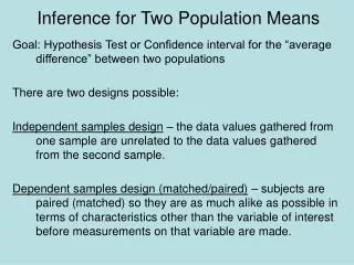
Comparison of 2 Population Means. Goal: To compare 2 populations/treatments wrt a numeric outcome Sampling Design: Independent Samples (Parallel Groups) vs Paired Samples (Crossover Design) Data Structure: Normal vs Non-normal Sample Sizes: Large ( n 1 , n 2 >20) vs Small. Independent Samples.

E N D
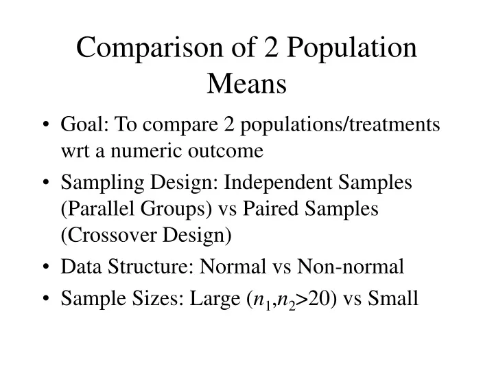
Comparison of 2 Population Means • Goal: To compare 2 populations/treatments wrt a numeric outcome • Sampling Design: Independent Samples (Parallel Groups) vs Paired Samples (Crossover Design) • Data Structure: Normal vs Non-normal • Sample Sizes: Large (n1,n2>20) vs Small
Independent Samples • Units in the two samples are different • Sample sizes may or may not be equal • Large-sample inference based on Normal Distribution (Central Limit Theorem) • Small-sample inference depends on distribution of individual outcomes (Normal vs non-Normal)
Parameters/Estimates (Independent Samples) • Parameter: • Estimator: • Estimated standard error: • Shape of sampling distribution: • Normal if data are normal • Approximately normal if n1,n2>20 • Non-normal otherwise (typically)
Large-Sample Test of m1-m2 • Null hypothesis: The population means differ by D0 (which is typically 0): • Alternative Hypotheses: • 1-Sided: • 2-Sided: • Test Statistic:
Large-Sample Test of m1-m2 • Decision Rule: • 1-sided alternative • If zobsza ==> Conclude m1-m2 > D0 • If zobs < za ==> Do not reject m1-m2 = D0 • 2-sided alternative • If zobsza/2 ==> Conclude m1-m2 > D0 • If zobs -za/2 ==> Conclude m1-m2 < D0 • If -za/2 < zobs < za/2 ==> Do not reject m1-m2 = D0
Large-Sample Test of m1-m2 • Observed Significance Level (P-Value) • 1-sided alternative • P=P(z zobs) (From the std. Normal distribution) • 2-sided alternative • P=2P(z |zobs| )(From the std. Normal distribution) • If P-Value a, then reject the null hypothesis
Large-Sample (1-a)100% Confidence Interval for m1-m2 • Confidence Coefficient (1-a) refers to the proportion of times this rule would provide an interval that contains the true parameter value m1-m2 if it were applied over all possible samples • Rule:
Large-Sample (1-a)100% Confidence Interval for m1-m2 • For 95% Confidence Intervals, z.025=1.96 • Confidence Intervals and 2-sided tests give identical conclusions at same a-level: • If entire interval is above D0, conclude m1-m2 > D0 • If entire interval is below D0, conclude m1-m2 < D0 • If interval contains D0, do not reject m1-m2 = D0
Example: Vitamin C for Common Cold • Outcome: Number of Colds During Study Period for Each Student • Group 1: Given Placebo • Group 2: Given Ascorbic Acid (Vitamin C) Source: Pauling (1971)
2-Sided Test to Compare Groups • H0: m1-m2= 0 (No difference in trt effects) • HA: m1-m2≠ 0 (Difference in trt effects) • Test Statistic: • Decision Rule (a=0.05) • Conclude m1-m2> 0 since zobs = 25.3 > z.025= 1.96
95% Confidence Interval for m1-m2 • Point Estimate: • Estimated Std. Error: • Critical Value: z.025 = 1.96 • 95% CI: 0.30 ± 1.96(0.0119) 0.30 ± 0.023 (0.277 , 0.323) Entire interval > 0
Small-Sample Test for m1-m2Normal Populations (P. 538) • Case 1: Common Variances (s12 = s22 = s2) • Null Hypothesis: • Alternative Hypotheses: • 1-Sided: • 2-Sided: • Test Statistic:(where Sp2 is a “pooled” estimate of s2)
Small-Sample Test for m1-m2Normal Populations • Decision Rule: (Based on t-distribution with n=n1+n2-2 df) • 1-sided alternative • If tobsta,n ==> Conclude m1-m2 > D0 • If tobs < ta,n ==> Do not reject m1-m2 = D0 • 2-sided alternative • If tobsta/2 ,n ==> Conclude m1-m2 > D0 • If tobs -ta/2,n ==> Conclude m1-m2 < D0 • If -ta/2,n < tobs < ta/2,n ==> Do not reject m1-m2 = D0
Small-Sample Test for m1-m2Normal Populations • Observed Significance Level (P-Value) • Special Tables Needed, Printed by Statistical Software Packages • 1-sided alternative • P=P(t tobs) (From the tn distribution) • 2-sided alternative • P=2P(t |tobs| )(From the tn distribution) • If P-Value a, then reject the null hypothesis
Small-Sample (1-a)100% Confidence Interval for m1-m2 - Normal Populations • Confidence Coefficient (1-a) refers to the proportion of times this rule would provide an interval that contains the true parameter value m1-m2 if it were applied over all possible samples • Rule: • Interpretations same as for large-sample CI’s
Small-Sample Inference for m1-m2Normal Populations (P.529) • Case 2: s12 s22 • Don’t pool variances: • Use “adjusted” degrees of freedom (Satterthwaites’ Approximation) :
Example - Maze Learning (Adults/Children) • Groups: Adults (n1=14) / Children (n2=10) • Outcome: Average # of Errors in Maze Learning Task • Raw Data on next slide • Conduct a 2-sided test of whether mean scores differ • Construct a 95% Confidence Interval for true difference Source: Gould and Perrin (1916)
Example - Maze LearningCase 1 - Equal Variances H0: m1-m2 = 0 HA: m1-m2 0 (a = 0.05) No significant difference between 2 age groups
Example - Maze LearningCase 2 - Unequal Variances H0: m1-m2 = 0 HA: m1-m2 0 (a = 0.05) No significant difference between 2 age groups
Small Sample Test to Compare Two Medians - Nonnormal Populations • Two Independent Samples (Parallel Groups) • Procedure (Wilcoxon Rank-Sum Test): • Rank measurements across samples from smallest (1) to largest (n1+n2). Ties take average ranks. • Obtain the rank sum for each group (W1 ,W2 ) • 1-sided tests:Conclude HA: M1 > M2 if W2 W0 • 2-sided tests:Conclude HA: M1M2 if min(W1, W2) W0 • Values of W0 are given in many texts for various sample sizes and significance levels. P-values are printed by statistical software packages.
Normal Approximation (Supp PP5-7) • Under the null hypothesis of no difference in the two groups (let W=W1 from last slide): • A z-statistic can be computed and P-value (approximate) can be obtained from Z-distribution
Example - Maze Learning As with the t-test, no evidence of population group differences
Inference Based on Paired Samples (Crossover Designs) • Setting: Each treatment is applied to each subject or pair (preferably in random order) • Data: di is the difference in scores (Trt1-Trt2) for subject (pair) i • Parameter: mD - Population mean difference • Sample Statistics:
Test Concerning mD • Null Hypothesis: H0:mD=D0 (almost always 0) • Alternative Hypotheses: • 1-Sided:HA: mD > D0 • 2-Sided: HA: mDD0 • Test Statistic:
Test Concerning mD • Decision Rule: (Based on t-distribution with n=n-1 df) • 1-sided alternative • If tobsta,n ==> Conclude mD> D0 • If tobs < ta,n ==> Do not reject mD= D0 • 2-sided alternative • If tobsta/2 ,n ==> Conclude mD> D0 • If tobs -ta/2,n ==> Conclude mD< D0 • If -ta/2,n < tobs < ta/2,n ==> Do not reject mD= D0 Confidence Interval for mD
Example Antiperspirant Formulations • Subjects - 20 Volunteers’ armpits • Treatments - Dry Powder vs Powder-in-Oil • Measurements - Average Rating by Judges • Higher scores imply more disagreeable odor • Summary Statistics (Raw Data on next slide): Source: E. Jungermann (1974)
Example Antiperspirant Formulations Evidence that scores are higher (more unpleasant) for the dry powder (formulation 1)
Small-Sample Test For Nonnormal Data • Paired Samples (Crossover Design) • Procedure (Wilcoxon Signed-Rank Test) • Compute Differences di (as in the paired t-test) and obtain their absolute values (ignoring 0s) • Rank the observations by |di| (smallest=1), averaging ranks for ties • Compute W+ and W-, the rank sums for the positive and negative differences, respectively • 1-sided tests:Conclude HA: M1 > M2 if W- T0 • 2-sided tests:Conclude HA: M1M2 if min(W+, W-) T0 • Values of T0 are given in many texts for various sample sizes and significance levels. P-values printed by statistical software packages.
Normal Approximation (Supp PP18-21) • Under the null hypothesis of no difference in the two groups : • A z-statistic can be computed and P-value (approximate) can be obtained from Z-distribution
Example - Caffeine and Endurance • Subjects: 9 well-trained cyclists • Treatments: 13mg Caffeine (Condition 1) vs 5mg (Condition 2) • Measurements: Minutes Until Exhaustion • This is subset of larger study (we’ll see later) • Step 1: Take absolute values of differences (eliminating 0s) • Step 2: Rank the absolute differences (averaging ranks for ties) • Step 3: Sum Ranks for positive and negative true differences Source: Pasman, et al (1995)
Example - Caffeine and Endurance Original Data
Example - Caffeine and Endurance Absolute Differences Ranked Absolute Differences W+ = 1+2+4+6+7+8=28 W- = 3+5+9=17
Example - Caffeine and Endurance Under the null hypothesis of no difference in the two groups: There is no evidence that endurance times differ for the 2 doses (we will see later that both are higher than no dose)
SPSS Output Note that SPSS is taking MG5-MG13, while we used MG13-MG5
Data Sources • Pauling, L. (1971). “The Significance of the Evidence about Ascorbic Acid and the Common Cold,” Proceedings of the National Academies of Sciences of the United States of America, 11: 2678-2681 • Gould, M.C. and F.A.C. Perrin (1916). “A Comparison of the Factors Involved in the Maze Learning of Human Adults and Children,” Journal of Experimental Psychology, 1:122-??? • Jungermann, E. (1974). “Antiperspirants: New Trends in Formulation and Testing Technology,” Journal of the Society of Cosmetic Chemists 25:621-638 • Pasman, W.J., M.A. van Baak, A.E. Jeukendrup, and A. de Haan (1995). “The Effect of Different Dosages of Caffeine on Endurance Performance Time,” International Journal of Sports Medicine, 16:225-230