Download
1 / 36
380 likes | 757 Views
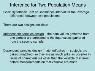
Comparing Two Population Means. Two kinds of studies or experiments. There are two general research strategies that can be used to compare the two populations of interest:

E N D
Two kinds of studies or experiments There are two general research strategies that can be used to compare the two populations of interest: • The two samples could be drawn from two independent populations (e.g. women and men, or patients taking drug A vs. those taking drug B) between subjects or independent samples design • The two sets of data could come from related populations (e.g. “before treatment” and “after treatment”, patient taking drug A and the SAME patient taking drug B at a later date, or subjects in different treatment groups are meaningfully matched according to some criteria)within subjects or dependent samples/matched pairs design We will focus on the independent samples case first.
Comparing Two Population Means: Using Independent Samples OBSERVATIONAL STUDY or EXPERIMENT? Observational Comparative Study • A research study in which two or more groups are compared with respect to some measurement or response. • The groups, determined by their natural characteristics, are merely “observed.”
Population 1m1 & s1 Population 2m2 & s2 Sample size = n1 Calculate: Sample size = n2 Calculate: Observational Comparative Study m1vs.m2 To make inferences use: Hypothesis test, CI for difference in means, effect size (d)
Example 1: Normal Human Body Temperature (females vs. males) • Is the normal human body temperature the same for females and males? • To answer this question two samples of size 65 are independently drawn from these two populations. • Let’s assume that our research hypothesis is that,for what ever reason,females have a higher mean body temperature than males.
Comparing Two Population Means: Using Independent Samples Comparative Experiment • A study in which two or more groups (see later) are randomly assigned to a “treatment” to see how the treatment affects some response. • If each experimental unit has the same chance of receiving any treatment, then the experiment is called a completely randomized design.
Randomly assign Treatment 1m1 & s1 Treatment 2m2 & s2 Sample size = n1 Calculate: Sample size = n2 Calculate: Comparative Experiment Population m1vs.m2 To make inferences use: Hypothesis test, CI for difference in means, effect size (d)
All possible questions in statistical notation In general, we can always compare two means by seeing how their difference (m1 – m2) compares to 0:
Hypotheses Note: If we wanted to establish that one mean was say e.g. at least 10 units larger than the other we could replace 0 in these statements by 10. In general to establish a difference of at least Dunits then we replace 0 by D. For testing equality Ho: m1 = m2 or (m1 – m2) = 0 The possible alternatives are: HA: m1 > m2 or (m1 – m2) > 0 (upper-tail) HA: m1 < m2 or (m1 – m2) < 0 (lower-tail) HA: 1 2 or (m1 – m2) 0 (two-tailed)
Example 1: Normal Human Body Temperature (females vs. males) Recall our research hypothesis is the females have a higher mean body temperature than males, therefore we have… mF = mean body temperature for females mM= mean body temperature for males Ho: mF = mM or equivalently (mF – mM) = 0 HA: mF > mM or equivalently (mF – mM) > 0
Test Statistic The basic form of the two-sample ttest statistic is... which assuming the following assumptions are satisfied has an approximate t-distribution (df(see 3 below)). • Both populations are approximately normally distributed. This assumption can be relaxed when both sample sizes (n1 and n2) are “large”. • Random, independent samples were drawn from the two populations of interest. • Thedf depends on how the standard error of the difference is estimated.
Yes, use pooled t-test No, use Welch’s t-test Test Statistic The standard error of the difference in sample means is calculated to different ways depending on whether or not we assume the population variances are equal. i.e., Can we assume ?
Estimate of the common variance (s2) Assuming equal population variances (pooled t-test) Estimate the standard error of the difference using the common pooled variance : where Then the sampling distribution is a t-distribution with n1+n2-2 degrees of freedom (df). Rule O’ Thumb:Assume variances are equal only if neither sample standard deviation is more than twice that of the other sample standard deviation.
Always round down! If variances of the measurements of the two groups are notequal (Welch’s t-test)... Estimate the standard error of the difference as: Then the sampling distribution is an approximate t distribution with a complicated formula for d.f.
Quantifying the Size of the Difference in Population Means (m1 – m2) To quantify the size of the effect, i.e. the difference in the population means we use… • Confidence Interval for (m1 – m2) (estimate) + (table value) SE(estimate) basic form • Effect Size (d)
Example 1: Normal Human Body Temperature (females vs. males) STEP 1) State Hypotheses mF = mean body temperature for females mM= mean body temperature for males Ho: mF = mM or equivalently (mF – mM) = 0 HA: mF > mM or equivalently (mF – mM) > 0
Example 1: Normal Human Body Temperature (females vs. males) STEP 2) Determine Test Criteria a) Choose a=.05 as a Type I Error is of little consequence. b) Use two-sample t-test, either pooled t-test or Welch’s t-test. As to which form to use we need to examine our data in terms of the equality of population variances. If uncertain use Welch’s!
Example 1: Normal Human Body Temperature (females vs. males) STEP 3) Collect Data and Compute Test Statistic Take independent samples from the two populations and examine the resulting data.
Example 1: Normal Human Body Temperature (females vs. males) Oneway Analysis > Means/Anova/Pooled t Populations appear normally distributed and our sample sizes are “large” (> 30). Few mild outliers for in sample for females Sample mean for females appears to slightly larger than that for males Variation appears to be similar for both samples. The sample standard deviation for females (sF = .74) is larger than that for males (sM = .70) although it is not twice as large, thus we assume pop. variances are equal.
Example 1: Normal Human Body Temperature (females vs. males) STEP 3) Collect Data and Compute Test Statistic Because it seems reasonable to assume the population variances are approximately equal we will use apooled t-test.
Pooled t-test calculations (FYI) For the body temperature example Assuming equal variances, the pooled estimate of common variance is So the standard error of the difference in sample means is
P-value = .0121 0 t = 2.28 Pooled t-test calculations (FYI) For the body temperature example Computing test statistic gives
Example 1: Normal Human Body Temperature (females vs. males) STEP 4) Compute p-value The p-value = .0121, which indicates we have a 1.21% chance of observing a difference in sample means this large by chance variation alone if in fact the population means were equal. STEP 5) Make Decision and Interpret Because p-value < .05 we reject Ho and conclude that the mean normal body temperature for females is larger than that for males.
Example 1: Normal Human Body Temperature (females vs. males) STEP 6) Quantify Significant Findings Construct a 95% CIfor (mF – mM) (98.39 – 98.10) + (1.98)(.127) = (.039o , .541o) We estimate the normal mean body temperature for women is between .039o F to .541o F larger than the normal mean body temperature for men.
Example 1: Normal Human Body Temperature (females vs. males) STEP 6) Quantify Significant Findings Effect Size (d) Thus effect size is moderate at best with % overlap of the two body temperature distributions being around 72.6%. Furthermore, the absolute difference represented by the lower confidence limit (LCL = .039 deg F) hardly seems of any physiological importance.
Power and Sample Size Issues(equal variance case) Power is a function of: • The sample sizes (n1 and n2), as the sample sizes increase so does power. • The smaller the common variance (s2) the larger the power. • The larger the difference (D) to detect the greater the power. • As always, as a increases the power increases.
Power and Sample Size Issues Common standard deviation to both populations/groups D = difference in population means which makes alternative true Common sample size (n1 = n2 = n) Probability of rejecting Ho when difference in means is D.
Power and Sample Size Issues Error Std. Dev = common standard deviation (s) = .721 for body temperature example. Difference in Means = D = |m1 – m2| = .29 which is the difference in the samples for body temperature example. Alpha = P(Type I Error) = .05 For body temperature example we have a power of 1 – b = .6240.
Power and Sample Size Issues Error Std. Dev = common standard deviation (s) = .721 for body temperature example. Difference in Means = D = |m1 – m2| = .29 which is the difference in the samples for body temperature example. Alpha = P(Type I Error) = .05
Example 3: Gestational age of babies born to women with preeclampsia We wish to compare the mean gestational age (in weeks) of babies born to women with preeclampsia during pregnancy vs. those who had normal pregnancies. Data:Preeclampsia: 38, 32, 42, 30, 38,35, 32, 38, 39, 29, 29, 32Normal: 40, 41, 38, 40, 40, 39, 39, 41, 41, 40, 40, 40
Example 3: Gestational age of babies born to women with preeclampsia The sample standard deviations control the slope of the reference lines, the line for preeclamptics is over 4 times steeper. The SD for the preeclamptic group is over 4 times larger!!
Example 3: Gestational age of babies born to women with preeclampsia Formally testing equality of variances: Test Statistic:
Example 3: Gestational age of babies born to women with preeclampsia F = (4.40)2/(.900)2 = 23.89 i.e. the sample variance for the preeclamptic group is 23.89 times larger than the sample variance for the normal pregnancy group. The p-value comes from an a F-dist. with numerator df = 11, denominator df = 11. We have strong evidence against equality of the variance of the response for these two populations of women (p < .0001) therefore we should not use a pooled t-Test!
F-distribution 0.8 0.6 Then the P-value < .0001 0.4 0.2 0.0 0 10 20 30 40 Let’s say our observed value for F was F0 = 23.89 F-distribution When H0 is true, the F-ratio ~ F(df1,df2) For example, consider the F-distribution with 11 and 11 df
Example 3: Gestational age of babies born to women with preeclampsia Oneway Analysis > t Test (i.e. non-pooled t–Test) We strong evidence that the mean gestational age of babies born to preeclamptic mothers is lower than that for babies born to women with normal pregnancies (p = .0013). Furthermore, we estimate that the mean gestational age for babies born to preeclamptic mothers is between 2.59 and 8.24 weeks less than the mean gestational age for babies born to mothers with normal pregnancies.
Summary • If in doubt, use non-pooled t-Test. • Be sure to quantify significant differences with a CI for (m1 – m2) or other measure of effect size. • Assess normality of both samples. When sample sizes are small, non-normality presents a problem and we should use test procedures that do not require normality (i.e. nonparametric tests, we’ll see these later).